We say that a sequence of estimators \(W_n\) is a consistent estimator for \(\theta \in \Theta\) if for every \(\epsilon>0\), and for every \(\theta \in \Theta\), the following holds \[\lim_{n\to \infty}\mbox{P}_{\theta}\left(|W_n - \theta|<\epsilon \right) = 1.\] The statement can also be equivalently written as \(\lim_{n\to \infty}\mbox{P}_{\theta}\left(|W_n - \theta|\ge \epsilon \right) = 0\) and by the Chebychev’s inequality, we have \[\mbox{P}_{\theta}\left(|W_n - \theta|\ge \epsilon \right) \le \frac{\mbox{E}_{\theta}(W_n-\theta)^2}{\epsilon^2}.\]
Therefore, a sufficient condition for an estimator \(W_n\) to be consistent estimator for \(\theta\) is to test whether \(\mbox{E}_{\theta}(W_n-\theta)^2 \to 0\) as \(n\to \infty\) for every \(\theta \in \Theta\).
In addition, we have the following well known decomposition, given by \[\mbox{E}_{\theta}(W_n-\theta)^2 = \mbox{Var}_{\theta}(W_n) + \left(\mbox{Bias}_{\theta}W_n\right)^2.\] Therefore, we have the following theorem:
for every \(\theta \in \Theta\), then \(W_n\) is a sequence of consistent estimators of \(\theta\).
It is important to note that the sequence of estimators must have finite variance which is not a necessary condition to be consistent. One can construct a different sequence of consistent estimators as well by virtue of the following theorem:
Many consistent estimators
If \(W_n\) is a consistent sequence of estimators of a parameter \(\theta\). Let \((a_n)\) and \((b_n)\) are sequence of real numbers satisfying \(\lim_{n\to \infty} a_n = 1\) and \(\lim_{n\to\infty} b_n = 0\). Then the sequence \(U_n = a_n W_n + b_n\) is a consistent sequence of estimators of \(\theta\).
The proof is simple and reader is encouraged to show this. Compute \(Var_{\theta}U_n\) and \(\mbox{Bias}_{\theta}U_n\) and show that these quantities converges to \(0\) as \(n\to \infty\).
13.1.1 Examples of consistent estimator using R
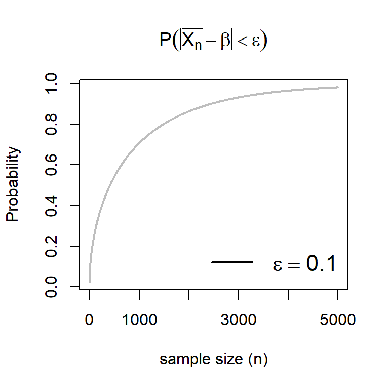
Using the software , we can demonstrate that \[\mbox{P}\left(\left|\overline{X_n}-\beta\right|<\epsilon\right)\to 0\] as \(n\to \infty\) for every choice of \(\epsilon >0\) and for all \(\beta\in(0,\infty)\). In the following code, we compute the above probability which is basically the integration \[\int_{n(\beta - \epsilon)}^{n(\beta +\epsilon)} \frac{e^{-\frac{y}{\beta}}y^{n-1}}{\Gamma(n)\beta^n}I_{(0,\infty)}(y)dy.\] We use the function pgamma() to compute the probabilities \(\mbox{P}(Y\le n(\beta \mp \epsilon))\) where \(Y\sim \mathcal{G}(\alpha = n, \beta)\).
Figure 13.1: As the sample size increases, the probability converges to 1. Students are encouraged to experiment with different choices of \(\beta\) and \(\epsilon\).
The Python code for computing the probability is attached below. We use gamma.cdf function to calculate probabilities which works similar to pgamma in R.
13.2 Large Sample Approximation of Variance of Estimators
Limiting Variance
For an estimator \(T_n\), if \[\lim_{n\to \infty} k_n Var (T_n) =\tau^2 <\infty,\] where \(\{k_n\}\) is a sequence of constants, then \(\tau^2\) is called the limiting variance or limit of variances.
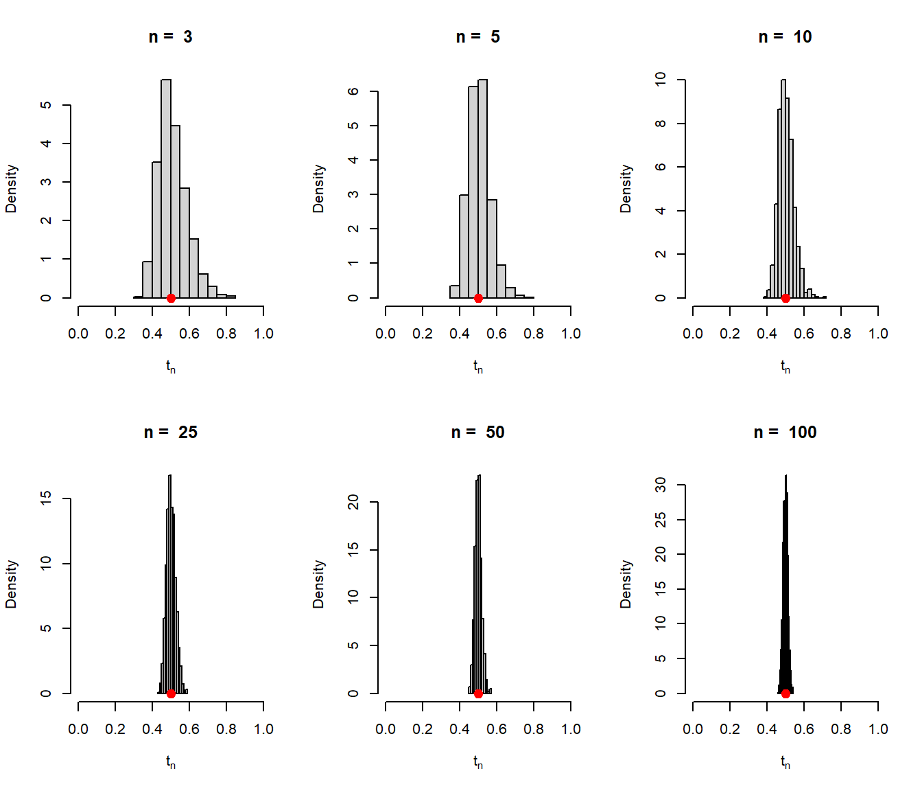
n_vals =c(3, 5, 10, 25, 50, 100)mu =2# true mean valuerep =1000# number of replicationssigma =0.5# population sd (given)par(mfrow =c(2,3))sample_means =numeric(length = rep)for(n in n_vals){ t_n =numeric(length = rep)for(i in1:rep){ x =rnorm(n = n, mean = mu, sd = sigma) sample_means[i] =mean(x) t_n[i] =1/mean(x) }hist(t_n, probability =TRUE, col ="lightgrey",xlab =expression(t[n]), main =paste("n = ", n),xlim =c(0,1))points(1/mu, 0, pch =19, col ="red", cex =1.4)}
The sampling distribution of \(1/\overline{X_n}\) is visualized using the histograms based on 1000 simulations for different sample size \(n\). As the sample size increases, the sampling distribution gets highly concentrated about the value \(1/\mu\).
The python code for visualizing the sampling distribution of \(\overline{X_n}^{-1}\) is provided beow.
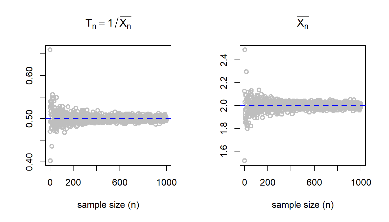
par(mfrow =c(1,2))n_vals =1:1000t_n =numeric(length =length(n_vals))sample_means =numeric(length =length(n_vals))for(n in n_vals){ x =rnorm(n = n, mean = mu, sd = sigma) sample_means[n] =mean(x) t_n[n] =1/mean(x)}plot(n_vals, t_n, col ="grey", lwd =2,xlab ="sample size (n)", main =expression(T[n]==1/bar(X[n])), ylab ="")abline(h =1/mu, col ="blue", lwd =2, lty =2)plot(n_vals, sample_means, col ="grey", lwd =2,xlab ="sample size (n)", main =expression(bar(X[n])), ylab ="")abline(h = mu, col ="blue", lwd =2, lty =2)
For large \(n\), as \(\overline{X_n}\) values becomes close to \(\mu\), then \(1/\overline{X_n}\) values get closer to \(1/\mu\) for \(\mu \ne 0\). In fact it shows that as \(n\to \infty\), \(1/\overline{X_n} \to 1/\mu\).
Python implementation of the convergence of the \(\overline{X_n}^{-1}\) to \(\frac{1}{\mu}\) is given below.
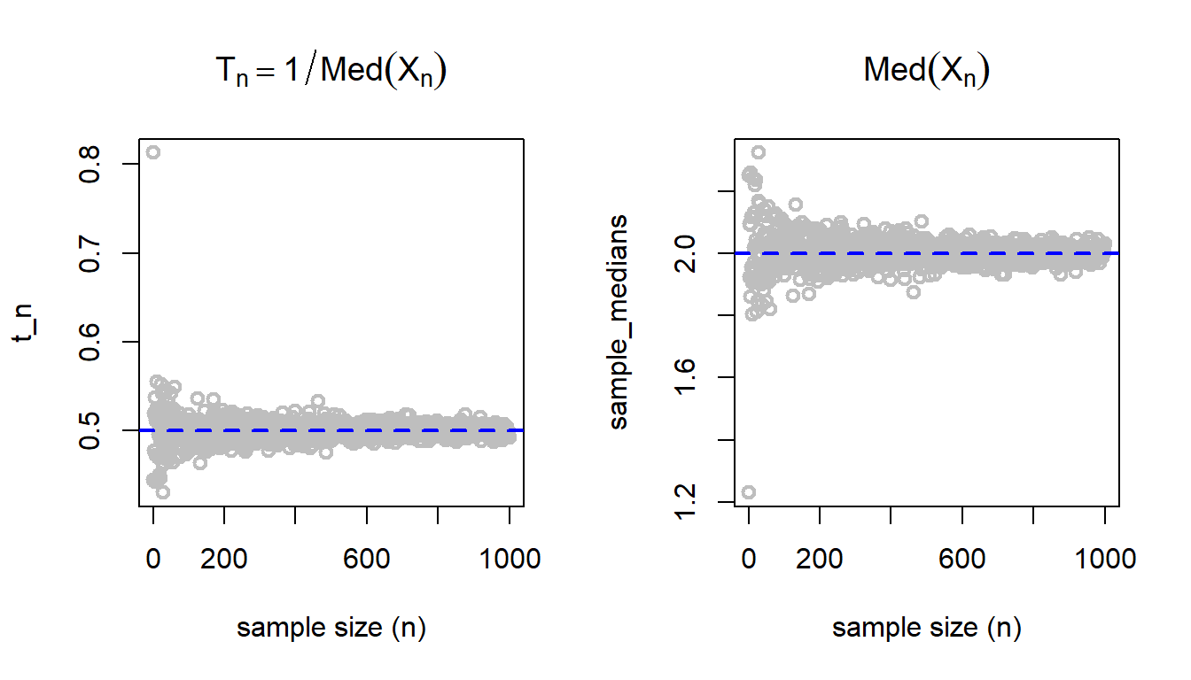
Instead of the sample mean, one may also aim to estimate \(1/\mu\) using the inverse of the sample median. For large \(n\), the approximations may be compared if we can compute the limiting variances of the inverse of the sample median. Before, going into any mathematical computations, first let us check how the estimator based on the sample median behaves for large \(n\) values.
par(mfrow =c(1,2))n_vals =1:1000t_n =numeric(length =length(n_vals))sample_medians =numeric(length =length(n_vals))for(n in n_vals){ x =rnorm(n = n, mean = mu, sd = sigma) sample_medians[n] =median(x) t_n[n] =1/median(x)}plot(n_vals, t_n, col ="grey", lwd =2,xlab ="sample size (n)", main =expression(T[n]==1/Med(X[n])))abline(h =1/mu, col ="blue", lwd =2, lty =2)plot(n_vals, sample_medians, col ="grey", lwd =2,xlab ="sample size (n)", main =expression(Med(X[n])))abline(h = mu, col ="blue", lwd =2, lty =2)
The inverse of the sample median also appears to be a consistent estimator for \(1/\mu\).
The python implementation of the above code for the convergence of \(\mbox{Med}(X_n)^{-1}\) to \(\frac{1}{\mu}\) is demonstrated below.
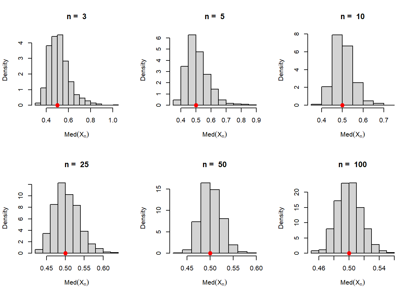
Now let us check, how the sampling distribution of the estimator of \(1/\mu\) based on the median, that is, \(1/\mbox{Med}(X_n)\) behaves for large \(n\) values.
n_vals =c(3, 5, 10, 25, 50, 100)mu =2rep =1000sigma =0.5par(mfrow =c(2,3))sample_medians =numeric(length = rep)for(n in n_vals){ t_n =numeric(length = rep)for(i in1:rep){ x =rnorm(n = n, mean = mu, sd = sigma) sample_medians[i] =median(x) t_n[i] =1/median(x) }hist(t_n, probability =TRUE, col ="lightgrey",xlab =expression(Med(X[n])), main =paste("n = ", n))points(1/mu, 0, pch =19, col ="red", cex =1.4)}
The python code for the sampling distribution of \(\mbox{Med}(X_n)^{-1}\) for different choices of \(n\) is shown below:
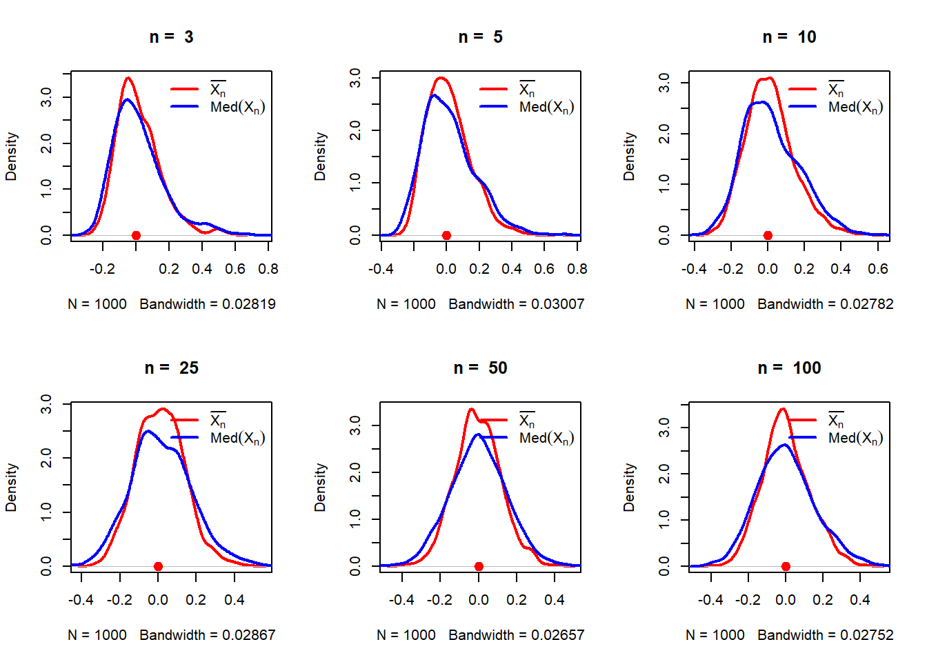
For the above simulation experiments, it appears that both inverse of the sample mean and the sample median appears to be a nice choice and both are approximately normally distribution for large \(n\). Let us now compare the inverse of the sample mean and sample median with respect to their asymptotic variances. We basically obtain the sampling distribution of the following two random variables for large \(n\) values.
\[\sqrt{n}\left(\frac{1}{\overline{X_n}}-\frac{1}{\mu}\right)\] and \[\sqrt{n}\left(\frac{1}{\mbox{Med}(X_n)}-\frac{1}{\mu}\right)\]
n_vals =c(3, 5, 10, 25, 50, 100)mu =2rep =1000sigma =0.5par(mfrow =c(2,3))sample_means =numeric(length = rep)sample_medians =numeric(length = rep)for(n in n_vals){ t_n =numeric(length = rep) # inverse of sample mean w_n =numeric(length = rep) # inverse of sample medianfor(i in1:rep){ x =rnorm(n = n, mean = mu, sd = sigma) t_n[i] =sqrt(n)*(1/mean(x) -1/mu) w_n[i] =sqrt(n)*(1/median(x) -1/mu) }plot(density(t_n), col ="red", lwd =2, main =paste("n = ", n))lines(density(w_n), col ="blue", lwd =2)legend("topright", legend =c(expression(bar(X[n])), expression(Med(X[n]))),col =c("red", "blue"), lwd =c(2,2), bty ="n")points(0, 0, pch =19, col ="red", cex =1.4)}
The simulation clearly demonstrates the comparison of the limiting variances of two estimators of \(1/\mu\).
Variance of the limit distribution of \(T_n\)
For an estimator \(T_n\), suppose that \[k_n\left(T_n - \tau(\theta)\right) \to \mathcal{N}(0,\sigma^2)\] in distribution. The parameter \(\sigma^2\) is called the asymptotic variance or variance of the limiting distribution of \(T_n\).
The python code for the comparison of the approximate sampling distribution for the large sample size \(n\) is shown below:
In the above problem \(T_n = \overline{X_n}^{-1}\) and \[\sqrt{n}\left(T_n - \frac{1}{\mu}\right) \to \mathcal{N}\left(0, \frac{\sigma^2}{\mu^4}\right).\] It is interesting to note that although the theoretical variance of \(T_n = \overline{X_n}^{-1}\), \(Var (T_n) = \infty\), but it has finite asymptotic variance \(\frac{\sigma^2}{\mu^4}\) for \(\mu\ne 0\), which is in fact more useful. The computation follows by a simple application of the Delta method, which gives \(Var (T_n) \approx \frac{\sigma^2}{n\mu^4}<\infty\).
Assymptotically efficient
A sequence of estimators of \(W_n\) is asymptotically efficient for a parameter \(\tau(\theta)\) if \[\sqrt{n}\left(W_n - \tau(\theta)\right) \to \mathcal{N}(0, v(\theta)),\] where \[v(\theta) = \frac{(\tau'(\theta))^2}{\mbox{E}_{\theta}\left(\left(\frac{\partial}{\partial \theta}\log f(X|\theta)\right)^2\right)},\] that is the asymptotic variance of \(W_n\) achieves the Cramer-Rao lower bound.
A natural question arises how to obtain an asymptotically efficient estimator, and we are lucky that the MLE is itself gives us algorithmic way of obtaining asymptotically efficient estimator. In the following section we discuss this in the light of an example.
13.3 MLE is asymptotically efficient
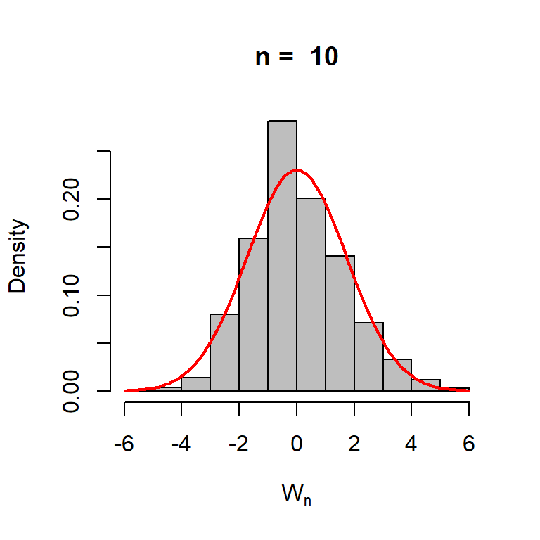
Suppose that \(X_1,\ldots,X_n\) be a random sample of size \(n\) from the Poisson distribution with parameter \(\lambda\). The Fisher Information is given by \(I(\lambda) = \lambda^{-1}\). The MLE of the parameter \(\lambda\) is given by \(\widehat{\lambda} = \overline{X_n}\). It can be easily shown by CLT that \[\sqrt{n}\left(\overline{X_n} - \lambda\right) \to \mathcal{N}(0, \lambda),\] in distribution, therefore, the asymptotic variance of \(\overline{X_n}\) is \(\lambda\), in fact, it is exact variance as well (why?). Let us perform some simulation experiment to see whether the claim is indeed true or not.
lambda =3rep =1000n =10w_n =numeric(length = rep)for(i in1:rep){ x =rpois(n = n, lambda = lambda) w_n[i] =sqrt(n)*(mean(x) - lambda)}hist(w_n, probability =TRUE, col ="grey",main =paste("n = ", n), xlab =expression(W[n]))curve(dnorm(x, mean =0, sd =sqrt(lambda)), add =TRUE,col ="red", lwd=2)
The experiment can be carried out for different choices of \(n\). The overlaying of the normal distriubtion with the asymptotic variance agrees with the theoretical claim.
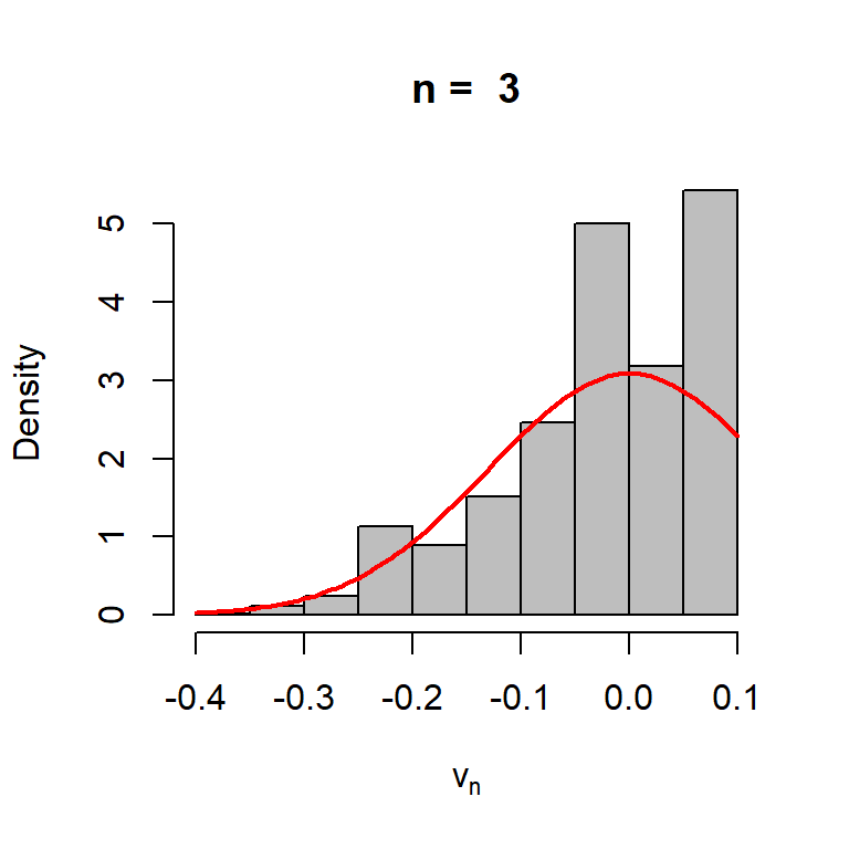
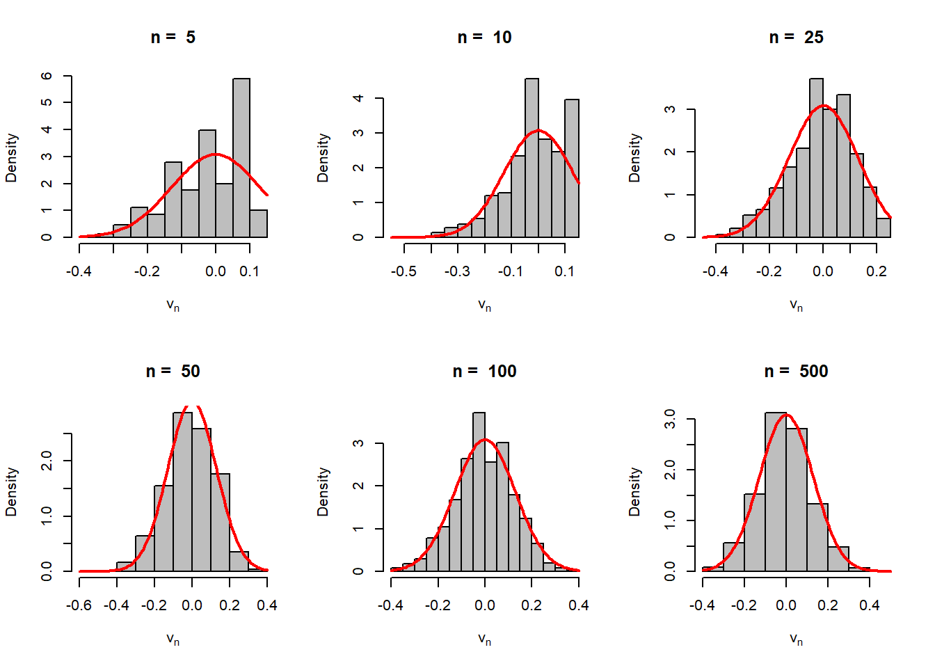
The above idea can be extended for estimating any continuous function of \(\lambda\) as well, say \(h(\lambda)\). We start with a concrete example. Suppose, we are interested in estimating \[h(\lambda) = \mbox{P}(X=2) = \frac{e^{-\lambda}\lambda^2}{2}.\] Therefore, the estimator is given by \[h(\widehat{\lambda}) = e^{-\overline{X_n}}\left(\overline{X_n}^2\right)/2,\] which is a highly nonlinear function of \(\overline{X_n}\). The theory suggests that \[\sqrt{n}\left(h(\widehat{\lambda})-h(\lambda)\right) \to \mathcal{N}(0,v(\lambda)),\] in distribution where \[v(\lambda) = \frac{(v'(\lambda))^2}{I(\lambda)} = \frac{\lambda^3e^{-2\lambda}(2-\lambda)^2}{4}.\]
h =function(lambda){ lambda^2*exp(-lambda)/2}lambda =3rep =1000n =3v_n =numeric(length = rep)for(i in1:rep){ x =rpois(n = n, lambda = lambda) v_n[i] =sqrt(n)*(h(mean(x)) -h(lambda))}hist(v_n, probability =TRUE, col ="grey",main =paste("n = ", n), xlab =expression(v[n]))curve(dnorm(x, mean =0, sd =sqrt(lambda^3*exp(-2*lambda)*(2-lambda)^2/4)), add =TRUE,col ="red", lwd=2)
The sample size is small, therefore, the histogram is not a good approximation of the normal distribution. The reader is encouraged to do the simulation with different values of \(n\).
n_vals =c(5,10,25,50, 100, 500)par(mfrow =c(2,3))for(n in n_vals){ v_n =numeric(length = rep)for(i in1:rep){ x =rpois(n = n, lambda = lambda) v_n[i] =sqrt(n)*(h(mean(x)) -h(lambda)) }hist(v_n, probability =TRUE, col ="grey",main =paste("n = ", n), xlab =expression(v[n]))curve(dnorm(x, mean =0, sd =sqrt(lambda^3*exp(-2*lambda)*(2-lambda)^2/4)), add =TRUE, col ="red", lwd=2)print(var(v_n))}
[1] 0.01110987
[1] 0.01362831
[1] 0.01436998
[1] 0.01733509
[1] 0.01544941
As the sample size increases, the approximation to the normal distribution is cleraly visible with the variance equal to the asymptotic variance.
[1] 0.01579456
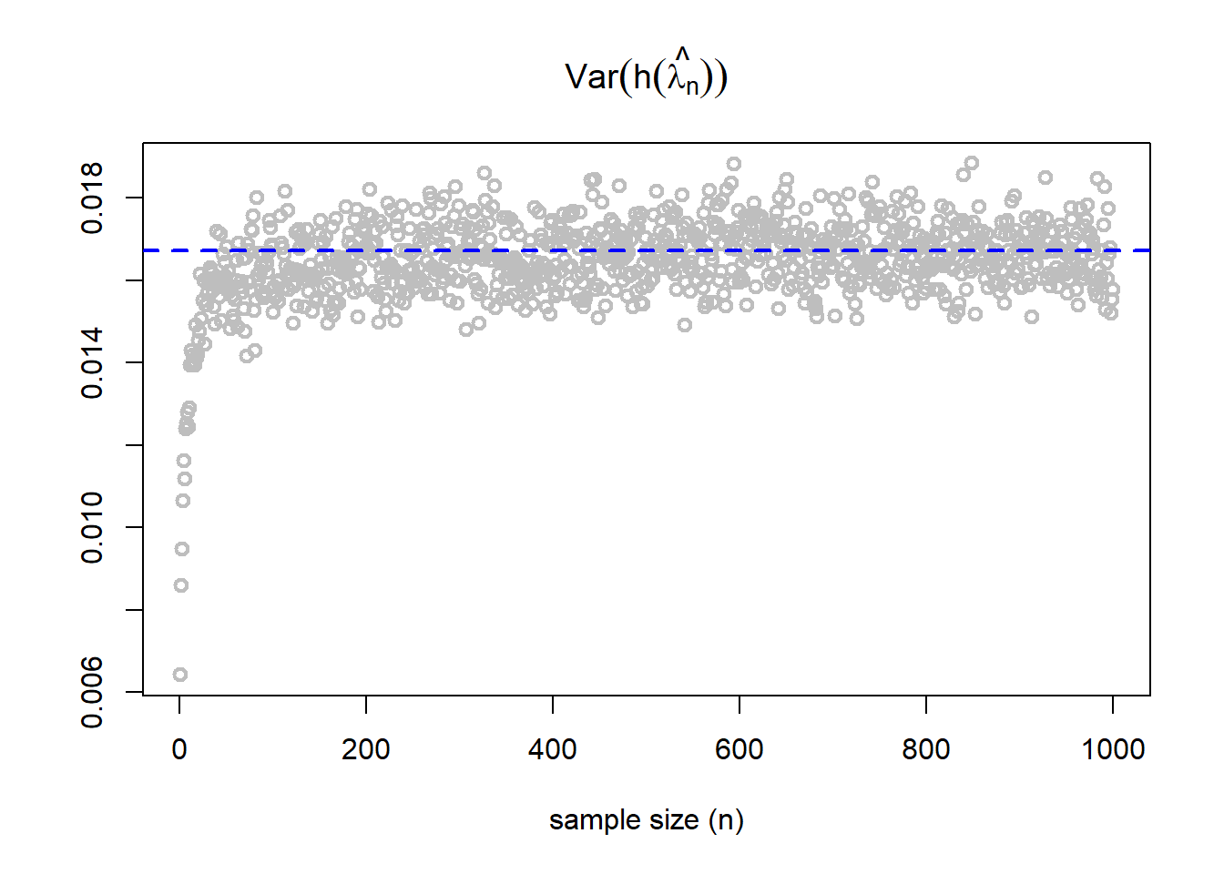
In the following, we numerically (through simulation) verify that how accurate the approximation of the variance by plugging in the \(\widehat{\lambda}\) in place of \(\lambda\).
\[\begin{eqnarray}
Var\left(h\left(\widehat{\lambda}\right)|\lambda\right) &\approx & \frac{(h'(\lambda))^2}{I_n(\lambda)}\\
&=& \frac{(h'(\lambda))^2}{\mbox{E}_{\lambda}\left(-\frac{\partial^2}{\partial \lambda^2}\log \mathcal{L}(\theta|\mathbf{X})\right)} \\
&\approx & \frac{\left[h'(\widehat{\lambda})\right]^2}{-\frac{\partial^2}{\partial \lambda^2}\log \mathcal{L}(\theta|\mathbf{X})|_{\lambda = \widehat{\lambda}}}.
\end{eqnarray}\] In the above computation, two approximations have been carried out. In the first approximation the computation of the asymptotic variance has been carried out by the first order Taylor’s approximation whereas in the second approximation, the expectation has been approximated by plugging in the MLE at the Fisher Information.
par(mfrow =c(1,1))n_vals =1:1000asym_var = lambda^3*exp(-2*lambda)*(2-lambda)^2/4var_v_n =numeric(length =length(n_vals))for(n in n_vals){ v_n =numeric(length = rep)for(i in1:rep){ x =rpois(n = n, lambda = lambda) v_n[i] =sqrt(n)*(h(mean(x)) -h(lambda)) } var_v_n[n] =var(v_n)}plot(n_vals, var_v_n, type ="p", col ="grey",lwd=2, xlab ="sample size (n)", ylab ="",main =expression(Var(h(hat(lambda[n])))))abline(h = asym_var, lty =2, col ="blue",lwd =2)
As the sample size increases, the approximated variance is close to the asymptotic variance. The asymptotic variance is shown using the dotted blue color line.
Based on the discussion about the optimal properties of the MLE, we have the following theorem:
Asymptotic efficiency of MLE
Let \(X_1,\ldots,X_n,\ldots\) be iid \(f(x|\theta)\), let \(\widehat{\theta}\) denote the MLE of \(\theta\), and let \(\tau(\theta)\) be a continuous function of \(\theta\). Under the regularity conditions on \(f(x|\theta)\), and, hence on \(\mathcal{L}(\theta|\mathbf{x})\), the likelihood function, \[\sqrt{n}\left(\tau(\widehat{\theta})-\tau(\theta)\right) \to \mathcal{N}(0,v(\theta)),\] where \(v(\theta)\) is the Cramer-Rao Lowe Bound. That is, \(\tau(\widehat{\theta})\) is a consistent and asymptotically efficient estimator of \(\tau(\theta)\).
13.4 Statistical Model for Contaminated data
Suppose that we have a random sample of size \(n\) from the normal distribution with mean \(\mu\) and variance \(\sigma^2\). However, there is a contamination with some values from the other distribution as well.
Consider the statistical model for the data with contamination as \[ X\sim \begin{cases} \mathcal{N}(\mu, \sigma^2),~~\mbox{with probability } 1-\delta \\
f(x),~~~~~\mbox{with probability } \delta.
\end{cases}\]
In the following we simulate a random sample of size \(n\) from the distribution with \(100\delta\%\) contamination.
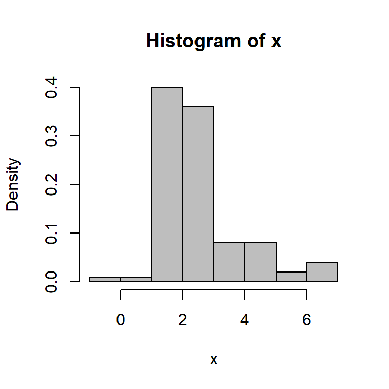
mu =2sigma2 =0.5theta =5tau2 =0.5delta =0.1n =100x =numeric(length = n)for(i in1:n){if(rbinom(n =1, size =1, prob =1-delta)==1) x[i] =rnorm(n =1, mean = mu, sd =sqrt(sigma2))else x[i] =rnorm(n =1, mean = theta, sd =sqrt(tau2))}hist(x, probability =TRUE, col ="grey")
Show that the mean and variance of \(\overline{X_n}\) is given by
\[Var\left(\overline{X_n}\right) = (1-\delta)\frac{\sigma^2}{n}+\delta \frac{\tau^2}{n}+\frac{\delta(1-\delta)(\theta-\mu)^2}{n}.\] If \(\theta\approx \mu\) and \(\sigma \approx \tau\), then \(Var(\overline{X_n}) \approx \frac{\sigma^2}{n}\), that means it achieves nearly optimal efficiency. However, the choice of \(f(x)\) plays a critical role. For example, if \(f(x)\) is Cauchy distribution, then the variance becomes infinite. You are encouraged to do some simulation considering the Cauchy distribution and plot the sampling distribution of \(\overline{X_n}\) for different choices of \(\delta\).
Breakdown value
Let \(X_{(1)}<X_{(2)}<\cdots<X_{(n)}\) be an ordered sample of size \(n\), and let \(T_n\) be a statistic based on this sample. \(T_n\) has breakdown value \(b,0\le b\le 1\), if for every \(\epsilon>0\), \[\lim_{X_{(\{(1-b)n\})}\to \infty} T_n <\infty~~~~~~\mbox{and}~~~~~\lim_{X_{(\{(1-(b+\epsilon))n\})}\to \infty} T_n =\infty\]
The sample mean \(\overline{X_n}\) has break down value 0.
The sample median \(M_n\) has breakdown value \(\frac{1}{2}\).
Trimmed mean
(Casella and Berger 2002) An estimator that splits the difference between the mean and median in terms of sensitivity is the \(\alpha-trimmed\) mean, \(0<\alpha<\frac{1}{2}\), defined as follows. \(\overline{X_n}^{\alpha}\), the \(\alpha-trimmed\) mean, is computed by deleting the \(\alpha n\) smallest observations and the \(\alpha n\) largest observations, and taking the arithmetic mean of the remaining observations.
Show that if \(T_n = \overline{X_n}^{\alpha}\), the \(\alpha\)-trimmed mean of the sample, \(0<\alpha<\frac{1}{2}\), show that \(0<b<\frac{1}{2}\).
13.4.1 Asymptotic normality of the \(M_n\)
Suppose that \(X_1,\ldots,X_n\) be a random sample of size \(n\) from the population density function \(f(x)\) with CDF \(F(x)\). Assume that the CDF is differentiable and median is \(\mu\), that is \(F(\mu) = \frac{1}{2}\).
Verify that, if \(n\) is odd, then \[\mbox{P}\left(\sqrt{n}(M_n-\mu)\le a\right) = \mbox{P}\left(\frac{\sum Y_i - np_n}{\sqrt{np_n(1-p_n)}} \ge \frac{(n+1)/2 - np_n}{\sqrt{np_n(1-p_n)}}\right)\]
Show that as \(n\to \infty\), \(p_n \to p = F(\mu) = \frac{1}{2}\) and \[\frac{(n+1)/2-np_n}{\sqrt{np_n(1-p_n)}} \to -2aF'(\mu) = -2af(\mu).\]
It is clear from the statement \[\mbox{P}\left(\sqrt{n}(M_n - \mu)\le a\right) \to \mbox{P}(Z\ge -2af(\mu))\] that \(\sqrt{n}(M_n -\mu)\) is asymptotically normal with mean 0 and variance \(\frac{1}{(2f(\mu))^2}\).
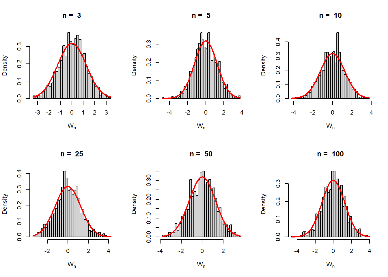
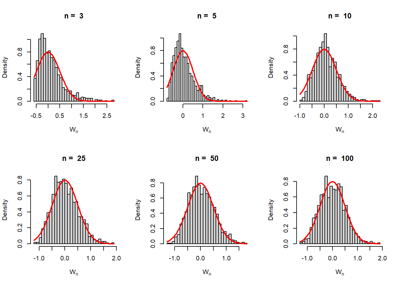
First let us understand the above result in terms of computer simulation and visualization. In the following we first perform the experiment with the sampling from the normally distributed population.
mu =2sigma2 =1f =function(x){dnorm(x, mean = mu, sd =sqrt(sigma2))}par(mfrow =c(2,3))n_vals =c(3,5,10,25,50, 100)rep =1000for (n in n_vals) { M_n =numeric(length = rep) W_n =numeric(length = rep)for(i in1:rep){ x =rnorm(n = n, mean = mu, sd =sqrt(sigma2)) M_n[i] =median(x) W_n[i] =sqrt(n)*(M_n[i] - mu) }hist(W_n, probability =TRUE, main =paste("n = ",n),xlab =expression(W[n]), breaks =30)curve(dnorm(x, mean =0, sd =sqrt(1/(4*f(mu)^2))),add =TRUE, col ="red", lwd =2)}
The sampling distribution of \(M_n\) is approximately normally distributed with asymptotic variance \(1/(2f(\mu))^2\). For simulation \(\mu=2\) and \(\sigma^2=1\) have been considered.
In the following, we perform the experiment with the exponential distribution with rate parameter \(\lambda\). The median of the exponential distribution is given by \(\mu = \frac{\ln 2}{\lambda}\). We simulate the distribution of \(\sqrt{n}\left(M_n - \frac{\ln 2}{\lambda}\right)\) for different values of \(n\) and as \(n\to \infty\), the normal approximation with the desired asymptotic variance is evident from the figures.
lambda =2mu =log(2)/lambdaf =function(x){dexp(x, rate = lambda)}par(mfrow =c(2,3))n_vals =c(3,5,10,25,50, 100)rep =1000for (n in n_vals) { M_n =numeric(length = rep) W_n =numeric(length = rep)for(i in1:rep){ x =rexp(n = n, rate = lambda) M_n[i] =median(x) W_n[i] =sqrt(n)*(M_n[i] - mu) }hist(W_n, probability =TRUE, main =paste("n = ",n),xlab =expression(W[n]), breaks =30)curve(dnorm(x, mean =0, sd =sqrt(1/(4*f(mu)^2))),add =TRUE, col ="red", lwd =2)}
The simulation has been carried from the exponential dsitribution with rate parameter \(\lambda = 2\), therefore, the true median is \(\mu= 0.3465736\).
Based on the above discussion, the students are encouraged to explore the ARE of the median to the mean, that is \(\mbox{ARE}\left(M_n,\overline{X_n}\right)\).
Show that \(\mbox{ARE}\left(M_n,\overline{X_n}\right)\) is unaffected by scale changes. This, it does not matter whether the underlying pdf if \(f(x)\) or \(\frac{1}{\sigma}f\left(\frac{x}{\sigma}\right)\).
Compute the \(\mbox{ARE}\left(M_n,\overline{X_n}\right)\) when the underlying distribution is Students’ \(t\) with \(\nu\) degrees of freedom, for \(\nu \in \{3,5,10,25,50,\infty\}\). What is your conclusion about the ARE and the tails of the distribution?
Compute the \(\mbox{ARE}\left(M_n,\overline{X_n}\right)\) when the underlying pdf is the Tukey model \[X\sim \begin{cases} \mathcal{N}(0,1)~~~~~~~\mbox{with probability } 1-\delta \\
\mathcal{N}(0,\sigma^2)~~~\mbox{with probability } \delta\end{cases}.\] Compute the ARE for a range of values of \(\delta\) and \(\sigma\). What can you conclude about the relative performance of the mean and the median?
13.5 Exercises
Suppose that we are interested in estimating the location parameter \(\mu\) for the normal, logistic and double exponential distribution based on a sample of size \(n\). Obtain \(\mbox{ARE}\left(M_n,\overline{X_n}\right)\) for each of the following distribution and discuss their comparative performance.
Suppose that \(X_1,X_2,\ldots,X_n\) be a random sample of size \(n\) from a population distribution characterized by the following probability density function \[f(x) = \begin{cases} \frac{\theta}{x^2}, ~~\theta<x<\infty\\
0,~~\mbox{otherwise},\end{cases}\] where \(\theta\in \Theta = (0,\infty)\) and we are interested in estimating the parameter \(\theta\). Obtain the maximum likelihood estimator of \(\theta\), call it \(\widehat{\theta_n}\). Check whether \(\widehat{\theta_n}\) is an unbiased estimator of \(\theta\). If not compute \(\mbox{Bias}_{\theta}\left(\widehat{\theta_n}\right)\) and check whether the estimator is asymptotically unbiased. Compute the mean squared error of the estimator \(\mbox{MSE}_{\theta}\left(\widehat{\theta_n}\right)\). Comment whether the estimator is asymptotically consistent or not.
Suppose that \(X_1, \ldots,X_n\) be a random sample of size \(n\) from a population following \(\mathcal{N}(\theta,\theta)\) distribution, where \(\theta>0\).
Show that the MLE of \(\theta\), \(\widehat{\theta_n}\) is a root of the quadratic equation \(\theta^2 +\theta - W = 0\), where \(W = \frac{1}{n}\sum_{i=1}^n X_i^2\), and determine which root is equals the MLE.
Find approximate variance of \(\widehat{\theta_n}\) using Delta method.
Suppose that \(Y_1,Y_2, \ldots,Y_n\) be a random sample of size \(n\) which satisfies the following equation \[Y_i = \beta X_i + \epsilon_i, ~i=1,2,\ldots,n,\] where \(X_1,\ldots,X_n\) are independent \(\mathcal{N}(\mu, \tau^2)\) random variables and \(\epsilon_1, \ldots,\epsilon_n\) are IID \(\mathcal{N}(0,\sigma^2)\), and \(X\)’s and \(\epsilon\)’s are independent. In terms of \(\mu, \tau^2\) and \(\sigma^2\), find the approximate means and variances for the following quantities:
\(\sum X_iY_i/\sum X_i^2\)
\(\sum Y_i /\sum X_i\)
\(\frac{1}{n}\sum(Y_i/X_i)\)
Write a simulation program in R to check the sampling distributions of the above quantities and experiment with different choices of \(\mu, \tau^2\) and \(\sigma^2\). Comment on your findings.
Consider the following hierarchical model \[\begin{eqnarray}
Y_n |W_n = w_n &\sim& \mathcal{N}\left(0, w_n + (1-w_n)\sigma_n^2\right) \\
W_n &\sim& \mbox{Bernoulli}(p_n).
\end{eqnarray}\] Show that for \(Y_n\), the limiting variance and the asymptotic variance differ.
Show that \(\mbox{E}(Y_n) = 0\) and \(Var(Y_n)=p_n+(1-p_n)\sigma_n^2\).
Show that \(\mbox{P}(Y_n) \to \mbox{P}(Z<a)\), where \(Z\sim \mathcal{N}(0,1)\) for any \(a\in \mathbb{R}\), and hence \(Y_n\to \mathcal{N}(0,1)\) in distribution.
Suppose that \(X_1,\ldots,X_n\) be iid observations from the normal distribution with mean \(\mbox{E}X=\mu\) and \(Var(X)=\sigma^2\). Show that for \(T_n = \frac{\sqrt{n}}{\overline{X_n}}\):
\(Var(T_n) = \infty\).
If \(\mu\ne 0\) and we delete the interval \((-\delta,\delta)\) from the sample space, then \(Var(T_n)<\infty\).
If \(\mu\ne 0\), then the probability content of the interval \((-\delta, \delta)\) approaches to \(0\) as \(n\to \infty\).
Suppose that \(X_1,\ldots,X_n\) be a random sample of size \(n\) from the Poisson(\(\lambda\)) distribution and we are interested in estimating the 0 probability. For example, the number of customers that come into a bank in a given time period is sometimes modeled as a Poisson random variable, and the 0 probability is the probability that no one enter the bank in one time period. If \(X\sim \mbox{Poisson}(\lambda)\), then \(\mbox{P}(X=0) = e^{-\lambda}\).
Consider the estimator of \(\tau = e^{-\lambda}\) as \(\hat{\tau} = \frac{1}{n}\sum_{i=1}^nY_i\), where \(Y_i = I(X_i=0)\). Show that \(\mbox{E}(\hat{\tau}) = e^{-\lambda}\) and \(Var(\hat{\tau}) = \frac{e^{-\lambda}(1-e^{-\lambda})}{n}\).
Consider another estimator of \(\tau\) as \(\tilde{\tau} = e^{-\hat{\lambda}}\), where \(\hat{\lambda}\) is the MLE of \(\lambda\). Obtain the asymptotic variance of \(\tilde{\tau}\).
Demonstrate using computer simulations that the following claims holds true (a) \(\sqrt{n}(\hat{\tau} - e^{-\lambda}) \to \mathcal{N}(0, e^{-\lambda}(1-e^{-\lambda}))\) and \(\sqrt{n}\left(\tilde{\tau} - e^{-\lambda}\right) \to \mathcal{N}\left(0, \lambda e^{-2\lambda}\right)\). Also report \(\mbox{ARE}\left(\hat{\tau}, \tilde{\tau}\right)\) and plot it as a function of \(\lambda\) and comment about your preferred estimator.
(Casella and Berger 2002) Suppose that \(X_1,X_2,\ldots,X_n\) are iid \(\mbox{Poisson}(\lambda)\). Find the best unbiased estimator of
\(e^{-\lambda}\), the probability \(X=0\)
\(\lambda e^{-\lambda}\), the probability \(X=1\).
For the best unbiased estimators in part (a) and (b), calculate the asymptotic relative efficiency with respect to the MLE. Which estimators do you prefer and why?
A preliminary test of a possible carcinogenic compound can be performed by measuring the mutation rate of microorganisms exposed to the compound. An experimenter places the compound in 15 petri dishes and record the following number of mutant colonies: \[10,7,8,13,8,9,5,7,6,8,3,6,6,3,5.\] Estimate \(e^{-\lambda}\), the probability that no mutant colonies emerge, and \(\lambda e^{-\lambda}\), the probability that one mutant colony will emerge. Calculate both the best unbiased estimator of and the MLE.
(Casella and Berger 2002) The performance of the sample mean in estimating the population may be compromised if there is a correlation in the sampling. This can seriously affect the properties of the sample mean. Suppose we introduce correlation in the sample \(X_1,\ldots,X_n \sim \mathcal{N}(\mu, \sigma^2)\), but \(X_i\)s are no longer independent.
For a equicorrelated case, that is, \(\mbox{Corr}(X_i,X_j)=\rho, i\ne j\), show that \[Var(\overline{X_n}) = \frac{\sigma^2}{n} + \frac{n-1}{n}\rho \sigma^2,\] so that \(Var(\overline{X_n})\not\to 0\) as \(n\to \infty\).
If the \(X_i\)’s are observed throught time (or distance), it is sometimes assumed that the correlation decreases with time (or distance), with one specific model being \(\mbox{Corr}(X_i,X_j) = \rho^{|i-j|}\). Show that the variance is given by \[Var(\overline{X_n}) = \frac{\sigma^2}{n}+\frac{2\sigma^2}{n^2}\frac{\rho}{1-\rho}\left(n - \frac{1-\rho^n}{1-\rho}\right),\] so that \(Var(\overline{X_n})\to 0\) as \(n\to \infty\).
The breakdown performance of the mean and the median continues with their scale estimate counterparts. For example \(X_1,\ldots,X_n\):
Show that the breakdown value of the sample variance \(S^2= \frac{1}{n-1}\sum_{i=1}^n\left(X_i - \overline{X_n}\right)^2\) is \(0\).
A robust alternative is the mean absolute deviation, or MAD, the median of \(|X_1-M|\), \(|X_2-M|,\ldots\),\(|X_n-M|\), where \(M\) is the sample median. Show that this estimator has a breakdown value \(50\%\).
Casella, George, and Roger L. Berger. 2002. Statistical Inference. 2nd ed. Pacific Grove, CA: Duxbury.