[1] 4 6 1 1 28 Method of Maximum Likelihood
8.1 A motivating example
We have a random sample \((X_1,X_2,\ldots,X_n)\) of size \(n\) from the \(\mbox{Geometric}(p)\) distribution, whose probability mass function is given by \[\mbox{P}(X=x) = (1-p)^{x-1}p,~x\in\{1,2,\ldots\}.\] The random variable \(X\) represents the number of throws required to obtain the first success if we continue tossing a coin with probability of head \(p\) until the first head is observed.
Suppose that a company produces a large number of identical coins. We are interested in estimating the probability of head. The following experimental procedure is planned to be followed to estimate the true probability of head. Out of a large number of coins \(n\) coins have been chosen and they are numbered as \(\{1,2,\ldots,n\}\). For each \(i\in\{1,2,\ldots,n\}\), \(i\)th coin has been kept on tossing till the first head appears. \(X_i\) denotes the number of throws required to observe the first head for the \(i\)th coin.
Suppose that \(n=5\) and the above experiment gave the following observations:
Let us compute the likelihood of observing the above sample as a function of \(p\) as follows: \[\mbox{P}\left(X_1 = 4, X_2=6, X_3 = 1, X_4 = 1, X_5 = 2\right) = (1-p)^9p^5.\] The sample space of \((X_1,\ldots,X_5)\) is given by the following set: \[\{1,2,3,\ldots\}^5=\{(x_1,x\ldots,x_5)\colon x_i\in \{1,2,3,\ldots\},1\le i\le5\}.\] Each of the points in this sample space has a positive probability of being included in the random sample of size \(5\). However, since the given sample is observed, is not unreasonable to consider that it has significantly larger likelihood. In other words, we ask the question, for what value of \(p\in(0,1)\), the probability of observing the given sample is as large as possible? To answer this, we can express the likelihood of given sample as a function of \(p\), which is here given by \[\mathcal{L}(p) = (1-p)^9\times p^5,~ p\in(0,1).\] We want to identify that for what value of \(p\), the likelihood of the observed sample is maximum, that is \(p^*\), so that \(\mathcal{L}(p^*)\ge \mathcal{L}(p)\) for all \(p\in(0,1)\). It boils down to a maximization problem. Instead of maximizing \(\mathcal{L}(\theta)\), we can maximize \(\log \mathcal{L}(\theta)\), which are referred as the likelihood and the log-likelihood function, respectively. \[l(p)=\log \mathcal{L}(p)=9\log(1-p)+5\log p.\] \[\frac{d}{dp}\left(\log \mathcal{L}(p)\right)= l'(p)=-\frac{9}{1-p}+\frac{5}{p}.\] Equating \(l'(p)=0\), we get \(p^*=\frac{5}{14}\) and it is easy to verify that \(l''(p^*)<0\).
par(mfrow = c(1,2))
p_star = 5/14
curve((1-x)^9*x^5, 0.01, 0.99, col = "red", lwd = 2,
      xlab = "p", ylab = "L(p)")
points(p_star, 0, pch = 19, col = "blue", cex = 1.4)
abline(v = p_star, col = "grey", lty = 2, lwd = 3)
curve(9*log(1-x) + 5*log(x), col = "red", lwd  = 2,
      xlab = "p", ylab = "l(p)")
points(p_star, 0, pch = 19, col = "blue", cex = 1.4)
abline(v = p_star, col = "grey", lty = 2, lwd = 3)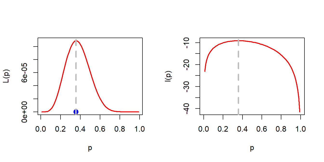
Based on the above data set, we obtained the estimate of the probability as \(\frac{5}{14}\). It is intuitively clear that this estimate is subject to uncertainty. By this statement, I essentially mean that if the this experiment would have been carried out by ten different individuals, then we would have obtained ten different samples of size \(5\). Certainly, the value of \(p^*\) is not expected to be the same for all the samples. Therefore, we are interested in computing the risk associated with this estimate. To formalize it further, let us try to obtain some explicit expression for \(p^*\).
Suppose that \(x_1,x_2,\ldots,x_n\) are realizations of the random sample \((X_1,X_2,\ldots,X_n)\). Then the likelihood function is given by \[\mathcal{L}(p) = \prod_{i=1}^n\mbox{P}(X_i=x_i)=(1-p)^{\sum x_i-n}p^n, 0<p<1,\] and the log-likelihood function is given by \[l(p)= \left(\sum x_i - n\right)\log(1-p)+n\log p.\] \(l'(p) = 0\) gives \(p^{*}=\frac{n}{\sum x_i} = (\overline{x_n})^{-1}\). Therefore the maximum likelihood estimator of \(p\) is given by \[\widehat{p_n} = \frac{1}{\overline{X_n}}.\] Our goal is to estimate the risk function \[\mathcal{R}(\widehat{p_n},p)=\mbox{E}\left(\frac{1}{\overline{X_n}} - p\right)^2, ~~p\in(0,1).\]
The likelihood and the log-likelihood
If \(X_1,X_2,\ldots,X_n\) be a random sample of size \(n\) from the population with PDF (PMF) \(f(x|\theta)\), then the likelihood function \(\mathcal{L}_n \colon \Theta \to [0,\infty)\) defined as \[\mathcal{L}_n(\theta) = \prod_{i=1}^nf\left(X_i|\theta\right), \theta \in \Theta.\] It is important to note that the likelihood function is the joint PDF (PMF), but considered as a function of \(\theta\), and certainly the statement \(\int_{\Theta}\mathcal{L}_n(\theta)d\theta=1\) not necessarily be true.
The log-likelihood function is defined by \[l_n(\theta) = \log \mathcal{L}_n(\theta), ~\theta \in \Theta.\]
8.1.1 Is the estimator consistent!
A desirable property of an estimator is that as the sample size increases, the sampling distribution of the estimator should be more concentrated about the true parameter value. We should not forget that an estimator is a random quantity which is subject to sampling variation. In this case, before going to some mathematical computation, we first check whether this is indeed happening or not for \(\widehat{p_n}\), the MLE of \(p\). We employed the following scheme to understand the behavior of \(\widehat{p_n}\) as \(n\to \infty\):
- Fix \(p_0\in(0,1)\)
- Fix sample size, \(n\in\{1,2,3,\ldots,1000\}\).
- For each \(n\in\{1,2,3,\ldots,1000\}\)
- Simulate \(X_1,\ldots,X_n \sim\mbox{Geometric}(p_0)\).
- Compute \(\overline{X_n}\)
- Compute \(\widehat{p_n} = \overline{X_n}^{-1}\).
- Plot the pairs \(\left(n,\widehat{p_n}\right), n\in\{1,2,\ldots,1000\}\).
- Do the above experiment for different choices of \(p_0\in(0,1)\).
p = 0.4
n_vals = 1:1000
pn_hat = numeric(length = length(n_vals))
for(n in n_vals){
  x = rgeom(n = n, prob = p)+1
  pn_hat[n] = 1/mean(x)
}
plot(n_vals, pn_hat, type = "l", col = "grey", lwd  = 2,
     xlab = "sample size (n)", ylab = expression(widehat(p[n])))
abline(h = 0.4, col = "blue", lwd = 3, lty = 2)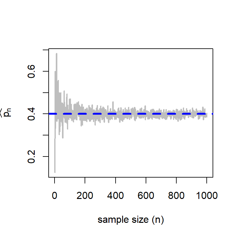
The statement can also be established theoretically. From the Weak Law of Large Numbers, we know that \(\overline{X_n} \to \mbox{E}(X)= \frac{1}{p}\) in probability as \(n\to \infty\). If we choose \(g(x) = \frac{1}{x}\), which is a continuous function, then \[g\left(\overline{X_n}\right) = \frac{1}{\overline{X_n}} = \widehat{p_n} \overset{P}{\to} p.\]
Continuous function and convergence in probability
If \(X_n \overset{P}{\to} X\), then \(g(X_n) \overset{P}{\to} g(X)\), where \(g(\cdot)\) is a continuous function.
8.2 Simulating the risk function of the MLE of \(p\)
The problem is to compute the risk function for different choices of \(p\in(0,1)\), \[\mathcal{R}\left(\overline{X_n}^{-1},p\right), 0<p<1.\]
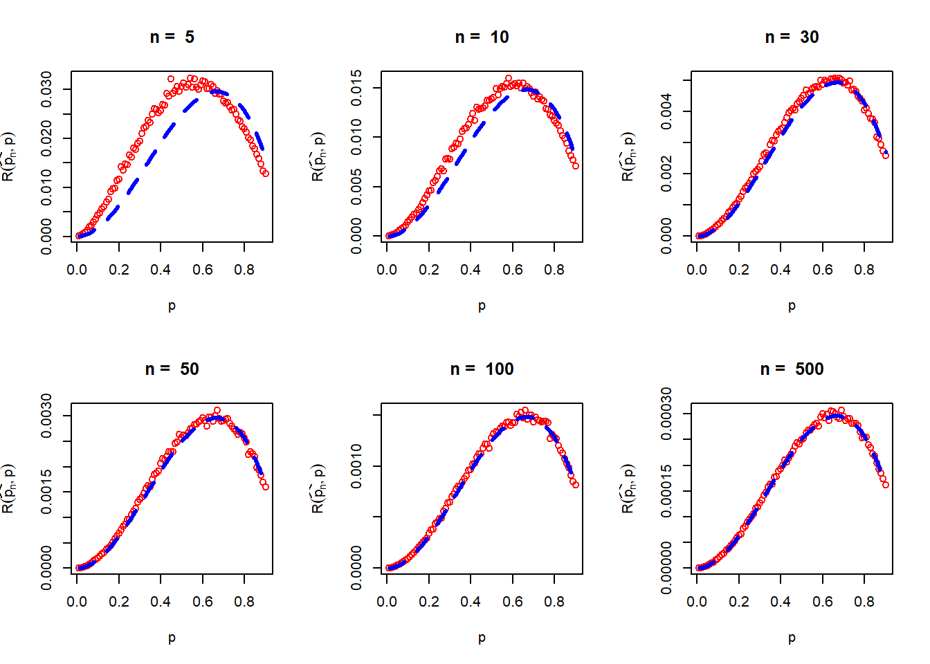
The following steps have been performed using R Programming to approximate the risk function of \(\overline{p_n}\) under the squared error loss function, which is also referred to as the Mean Squared Error (MSE) of \(\widehat{p_n}\).
- Discretize \((0,1)\) as \((p_1,\ldots,p_L)\).
- Fix sample size \(n\)
- Fix \(M\), the number of replications
- For each \(p\in \{p_1,\ldots,p_L\}\)
- For each \(m\in \{1,2,\ldots,M\}\)
- Simulate \(X_1, X_2,\ldots,X_n \sim \mbox{Geometric}(p)\).
- Compute loss \(l_m = \left(\frac{1}{\overline{X_n}}-p\right)^2\)
- Compute the risk \(\mathcal{R}\left(\frac{1}{\overline{X_n}},p\right)=\frac{1}{M}\sum_{m=1}^Ml_m\).
- For each \(m\in \{1,2,\ldots,M\}\)
- Plot the pairs of values \(\left\{p,\mathcal{R}\left(\frac{1}{\overline{X_n}},p\right)\right\}, p\in \{p_1,\ldots,p_L\}\).
- Repeat the above exercise for different choices of \(n\)
par(mfrow = c(2,3))
n_vals = c(5, 10, 30, 50, 100, 500)                  # different sample sizes
M = 5000                                             # number of replications
prob_vals = seq(0.01, 0.9, by = 0.01)
for(n in n_vals){
  risk_pn_hat = numeric(length = length(prob_vals))
  for(i in 1:length(prob_vals)){
    p = prob_vals[i]
    loss_pn_hat = numeric(length = M)
    for(j in 1:M){
      x = rgeom(n = n, prob = p) + 1
      loss_pn_hat[j] = (1/mean(x)-p)^2               # compute loss
    }
    risk_pn_hat[i] = mean(loss_pn_hat)               # compute risk (average loss)
  }
  plot(prob_vals, risk_pn_hat, col = "red", xlab = "p",
       ylab = expression(R(widehat(p[n]),p)),
       main = paste("n = ", n))
  lines(prob_vals, prob_vals^2*(1-prob_vals)/n,
        col = "blue", lwd = 3, lty = 2)              # add true risk function
}
For this problem it is almost impossible to compute the risk function analytically. Let us try to obtain an approximation of the risk function which performs well for large \(n\). Consider \(g\left(x\right)=\frac{1}{x}\). Expanding the Taylor’s Polynomial of \(g(\overline{X_n})\) about \(\frac{1}{p}\) gives
\[\begin{aligned} g\left(\overline{X_n}\right)&\approx& g\left(\frac{1}{p}\right) + \left(\overline{X_n}-\frac{1}{p}\right)g'\left(\frac{1}{p}\right)\\ &\approx& p+\left(\overline{X_n}-\frac{1}{p}\right)\left(-p^2\right). \end{aligned} \tag{8.1}\]
From the Central Limit Theorem we have \[\overline{X_n}\overset{a}{\sim}\mathcal{N}\left(\frac{1}{p},\frac{1-p}{p^2n}\right),\] therefore, for large \(n\), \(Var\left(\overline{X_n}\right) \approx \frac{1-p}{p^2n}\). Taking expectation on both sides of the Taylor’s polynomial we see that \[\mbox{E}\left[g\left(\overline{X_n}\right)\right] \approx p\] and the approximate risk is given by \[\mathcal{R}\left(\frac{1}{\overline{X_n}},p\right)= \mbox{E}\left(\frac{1}{\overline{X_n}}-p\right)^2\approx \mbox{E}\left(\overline{X_n}-\frac{1}{p}\right)^2(-p^2)^2\approx Var\left(\overline{X_n}\right)p^4=\frac{(1-p)p^2}{n}.\] Therefore \[\mathcal{R}\left(\frac{1}{\overline{X_n}},p\right) \approx \frac{(1-p)p^2}{n}, ~~\mbox{for large }n.\] In the Fig, the simulated risk function is overlaid with the approximate risk function obtained the Taylor’s approximation (first order). It can be noted that for large \(n\), the approximations are remarkable close to the true risk function.
It is interesting to observe that the risk is different at different values of the parameter \(p\). Therefore, if the estimate of the parameter is \(p^*\), then the estimated risk will be \(\frac{(1-p^*)p^*{^2}}{n}\), which is approximately equal to \(\frac{0.082}{n}\) for \(p^*=\frac{5}{14}\) and \(n=5\). However, one may possibly want to get an upper bound of the risk which is independent of the choices of \(p\), which can be obtained by maximizing the risk function with respect to \(p\).
\[\frac{d}{dp}\left[\frac{(1-p)p^2}{n}\right] = \frac{2p-3p^2}{n}=0\] gives \(p^*=\frac{2}{3}\). Therefore, \[\max_{p\in(0,1)}\mathcal{R}\left(\overline{X_n}^{-1},p\right)=\frac{\left(1-\frac{2}{3}\right)\left(\frac{2}{3}\right)^2}{n}=\frac{4}{27n}.\] Therefore, for large \(n\) \[\mathcal{R}\left(\overline{X_n}^{-1},p\right)\le \frac{4}{27n},~\mbox{for all }p\in(0,1).\] One might ask the question that what would be the minimum required sample size so that the maximum risk would be less than some small number \(\epsilon = 0.001\) (say). From the inequality, we can obtain \(\frac{4}{27n}\le 0.001\) implies \(n\ge\frac{4}{27\times0.001}=148.1481\). Therefore, at least a sample size of \(n\ge 149\) would be required to ensure the accuracy of the estimate less than 0.001. A general formula can be written as \(n\ge \left[\frac{4}{27\epsilon}\right]+1\) for a given accuracy level \(\epsilon>0\), where \([x]\) represents the greatest integer \(\le x\).
8.2.1 A not so common discrete distribution
The discrete uniform distribution on the set \(\{1,2,\ldots,\theta\}\), where \(\theta\in\Theta = \{1,2,3,\ldots\}\) is given by \[\mbox{P}(X=x) = \begin{cases} \frac{1}{\theta}, x\in \{1,2,\ldots,\theta\} \\ 0,~~ \mbox{otherwise}. \end{cases}\] Suppose, we have a random sample of size \(n\), \((X_1,X_2,\ldots,X_n)\) are available and let \(Y_n = \max(X_1,\ldots,X_n)\). We are interested in estimating the parameter \(\theta\) which can take any value from the countable set \(\{1,2,\ldots\}\). The likelihood function is given by \[\mathcal{L}(\theta) = \begin{cases} \left(\frac{1}{\theta}\right)^n,~~\theta \in\{y_n, y_n+1,y_n+2,\ldots\} \\ 0,~~~\mbox{otherwise}\end{cases}\] In addition, it is easy to understand that the likelihood function attains it’s maximum at \(y_n\).
theta = 6
n = 5
x = sample(1:theta, size = n, replace = TRUE)
y_n = max(x)
Lik = function(theta){
  if(theta<y_n)
    return(0)
  if(is.integer(theta) && theta>=y_n)
    return(theta^(-n))
}
theta_vals = 1:10
Lik_vals = numeric(length = length(theta_vals))
for(i in 1:length(theta_vals)){
  Lik_vals[i] = Lik(theta = theta_vals[i])
}
plot(theta_vals, Lik_vals, type = "h", pch = 19, col = "grey",
     cex = 1.4, ylab = expression(L(theta)), xlab = expression(theta))
points(theta_vals, Lik_vals, pch = 19, col = "blue", cex = 1.3)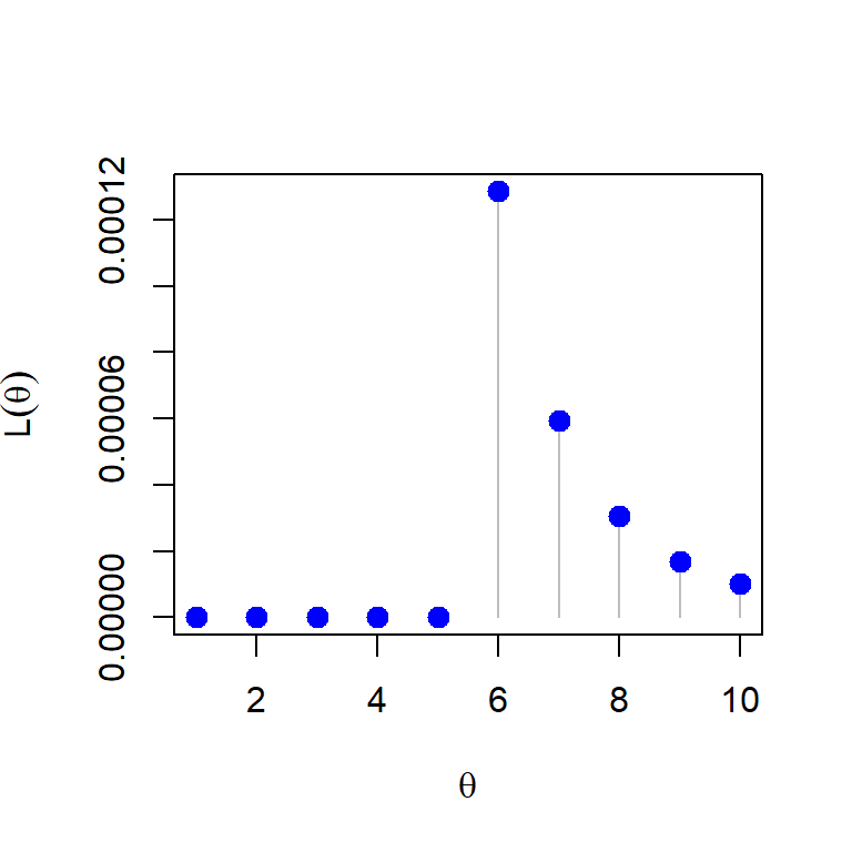
8.3 An experiment with the continuous distribution
Suppose that we have a random sample \((X_1,\ldots,X_n)\) of size \(n\) from the exponential distribution with rate parameter \(\lambda\). Let \(X\sim \mbox{Exponential}(\lambda)\) be the population distribution and the parameter space is \(\Theta =(0,\infty)\). We are interested in estimating the probability \(\mbox{P}(X\le 1)\).
First we make the observation that the desired quantity \(\psi=\mbox{P}(X\le1)\) is a function of \(\lambda\), which is given by \[\psi = \int_0^1 \lambda e^{-\lambda x}dx = 1 - e^{-\lambda}.\] The original parameter \(\lambda\in (0,\infty)\), which implies that \(\psi \in (0,1)\). As \(\lambda\to \infty\), \(\psi\to 1\) and as \(\lambda\to 0\), \(\psi \to 0\). Our aim is to estimate \(\psi\) based on the observations which is a function of \(\lambda\). Let us understand this problem step by step. First we need to estimate the parameter \(\lambda\) and then we can use it to approximate \(\psi\).
8.3.1 Computation of MLE of the parameter
Suppose that \((x_1, x_2, \ldots,x_n)\) be the collected sample of size \(n\): - The likelihood function is given by \[\mathcal{L}(\lambda)= f(x_1,x_2,\ldots,x_n|\lambda)=\prod_{i=1}^n\lambda e^{-\lambda x_i}.\] The function is explicitly written as \[\mathcal{L}(\lambda)= \begin{cases} \lambda^n e^{-\lambda\sum_{i=1}^nx_i},~~0<\lambda <\infty \\ 0,~~~~\mbox{otherwise.}\end{cases}.\] The log-likelihood function is \(l(\lambda) = \log \mathcal{L}(\lambda)\) is given by \[l(\lambda) = n\log \lambda - \lambda \sum_{i=1}^n x_i.\] Equating \(l'(\lambda)=0\), we obtain \(\lambda^*=\frac{n}{\sum_{i=1}^nx_i}=\frac{1}{\overline{x_n}}\), inverse of the sample mean. It is easy to see that \(l''(\lambda)<0\) for all \(\lambda \in (0,\infty)\), therefore, \(l''(\lambda^*)<0\). Therefore, the Maximum Likelihood Estimator (MLE) of the parameter \(\lambda\), based on a sample of size \(n\), is given by \[\widehat{\lambda_n}=\left(\overline{X_n}\right)^{-1}.\] Here I would like to make an extremely important point which many people miss. It is important to note that in the above discussion \(\lambda^*\) is a \(\texttt{fixed quantity}\) which is computed based on a single realization of the sample \((X_1,\ldots,X_n)\), whereas \(\widehat{\lambda_n}\) is a \(\texttt{random quantity}\) which can be characterized by a probability distribution.
8.3.2 Computation of MLE of the function of parameter
To obtain the estimator of \(\psi\), based on the above sample, a natural choice of the estimator of \(\psi\) is given by \[\widehat{\psi_n} = 1-e^{-\widehat{\lambda_n}},\] where \(\widehat{\lambda_n}\) is the MLE of \(\lambda\). The following observations we have:
- The MLE \(\widehat{\lambda}\) is a function of the sample mean \(\overline{X_n}\).
- For the sample mean \(\overline{X_n}\), we have large sample normal approximation due to the Central Limit Theorem. The underlying population has finite variance, therefore, CLT holds. It would be interesting to see whether the MLE \(\widehat{\lambda_n} = \frac{1}{\overline{X_n}}\), a function of \(\overline{X_n}\) follows some approximate distribution at least for large \(n\). Also, can this result be extended for \(\widehat{\psi_n}\), a nonlinear function of the MLE?
- By the WLLN, we know that \(\overline{X_n}\overset{P}{\to} \mbox{E}(X)\). Is it true that \(\widehat{\lambda_n}\overset{P}{\to}\lambda\) for all \(\lambda\in (0,\infty)\). Also, can this result be extended for \(\widehat{\psi_n}\), a nonlinear function of the MLE?
8.3.3 Convergence of Estimators \(\widehat{\lambda_n}\) and \(\widehat{\psi_n}\) for large \(n\)
Using the Weak Law of Large Numbers, we know that \[\overline{X_n} \overset{P}{\to}\mbox{E}(X) = \frac{1}{\lambda}.\] Our claim is that \[\widehat{\lambda_n}\overset{P}{\to} \lambda,~~~~~~~\widehat{\psi_n}\overset{P}{\to} \psi.\] Before going into the theoretical justifications, let us see by computer simulations, how these estimators behaves as the sample size \(n\) increases. We implement the following algorithm:
- Fix \(\lambda \in (0,\infty)\)
- Fix \(n\in\{1,2,\ldots,1000\}\)
- For each \(n\)
- Simulate \(X_1,X_2,\ldots,X_n \sim \mbox{Exponential}(\lambda)\)
- Compute \(\overline{X_n}\)
- Compute \(\widehat{\lambda_n} = \overline{X_n}^{-1}\)
- Compute \(\widehat{\psi_n} = 1- e^{-\widehat{\lambda_n}}\).
- Plot the pairs \(\left(n,\overline{X_n}\right), n\in \{1,2,\ldots,1000\}\)
- Plot the pairs \(\left(n,\widehat{\lambda_n}\right), n\in \{1,2,\ldots,1000\}\).
- Plot the pairs \(\left(n,\widehat{\psi_n}\right), n\in \{1,2,\ldots,1000\}\)
par(mfrow = c(1,3))
lambda = 2                                         # rate parameter
psi = 1-exp(-lambda)                               # true probability

n_vals = 1:1000                                    # increasing sample size
sample_means = numeric(length = length(n_vals))
lambda_hat = numeric(length = length(n_vals))
psi_hat = numeric(length = length(n_vals))

for(n in n_vals){
  x = rexp(n = n, rate = lambda)
  sample_means[n] = mean(x)
  lambda_hat[n] = 1/sample_means[n]                # estimate of the rate parameter
  psi_hat[n] = 1 - exp(-lambda_hat[n])             # estimate of the probability (psi)
}
plot(n_vals, sample_means, col = "red", ylab = "",
     type = "l", xlab = "sample size (n)",
     main = expression(bar(X[n])), cex.lab = 1.5,
     cex.main = 1.5)                               # Sampling distribution of MLE of lambda
abline(h = 1/lambda, lty = 2, col = "blue", lwd = 3)

plot(n_vals, lambda_hat, col = "red", ylab = "",   # Consistency of MLE of lambda
     type = "l", xlab = "sample size (n)",
     main = expression(widehat(lambda)), cex.lab = 1.5,
     cex.main = 1.5)
abline(h = lambda, lty = 2, col = "blue", lwd = 3)

plot(n_vals, psi_hat, col = "red", ylab = "",      # Consistency of MLE of psi
     type = "l", xlab = "sample size (n)",
     main = expression(widehat(psi[n]) == 1-e^{-widehat(lambda[n])}) , cex.lab = 1.5,
     cex.main = 1.5)
abline(h = psi, lty = 2, col = "blue", lwd = 3) 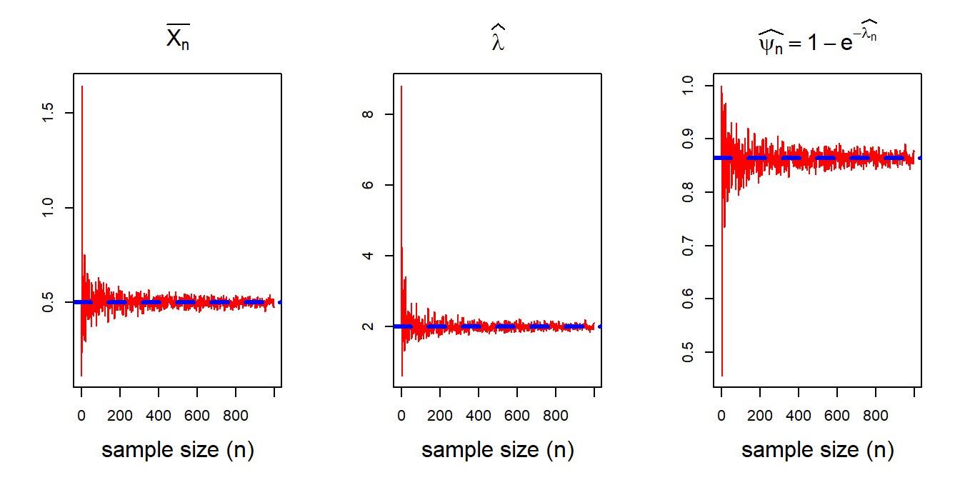
The figures clearly suggests that all the estimators converge to the true value as \(n\to \infty\). This is due to the fact that both \(\widehat{\lambda_n}\) and \(\widehat{\psi_n}\) are continuous transformation of \(\overline{X_n}\). Let us now look into the large sample approximation of the sampling distributions of \(\widehat{\lambda_n}\) and \(\widehat{\psi_n}\).
8.3.4 Large sample approximations
We recall that as the sample size \(n\to \infty\), \(\overline{X_n}\) can be well approximated by the normal distribution. More specifically, in our context, for large \(n\), \[\overline{X_n} \overset{a}{\sim} \mathcal{N}\left(\frac{1}{\lambda}, \frac{1}{\lambda^2n}\right)\] as for the given population \(\mbox{E}(X) = \frac{1}{\lambda}\) and \(Var(X) = \frac{1}{\lambda^2}\). Before going into some theoretical justifications, let us visualize the sampling distribution of \(\widehat{\lambda_n}\) and \(\widehat{\psi_n}\) for different choices (ascending order) of \(n\). The simulation scheme is already demonstrated for the \(\mbox{Geometric}(p)\) distribution in the previous section.
par(mfrow = c(1,3))
M = 1000                                   # number of replications
n = 500                                    # sample size
lambda = 2                                 # true rate parameter
sample_means = numeric(length = M)         # store sample means
lambda_hat = numeric(length = M)           # store MLEs of lambda
psi_hat = numeric(length = M)              # store MLEs of psi
for (i in 1:M) {
  x = rexp(n = n, rate = lambda)           # simulate from population
  sample_means[i] = mean(x)                # compute sample means
  lambda_hat[i] = 1/mean(x)                # compute MLE of lambda
  psi_hat[i] = 1 - exp(-lambda_hat[i])     # compute MLE of psi
}
hist(sample_means, probability = TRUE,
     main = paste("n = ", n), xlab = expression(bar(X[n])), cex.lab = 1.3)
curve(dnorm(x, mean = 1/lambda, sd = 1/sqrt(lambda^2*n)),
      add = TRUE, col = "red", lwd = 2)

hist(lambda_hat, probability = TRUE,
     main = paste("n = ", n), xlab = expression(widehat(lambda[n])), cex.lab = 1.3)
curve(dnorm(x, mean = lambda, sd = sqrt(lambda^2/n)),
      add = TRUE, col = "red", lwd = 2)

hist(psi_hat, probability = TRUE,
     main = paste("n = ", n), xlab = expression(g(widehat(lambda[n]))), cex.lab = 1.3)
points(psi, 0, pch = 19, col = "red",
       cex = 1.4)
curve(dnorm(x, mean = psi, sd = sqrt(lambda^2*exp(-2*lambda)/n)),
      add = TRUE, col = "red", lwd = 2)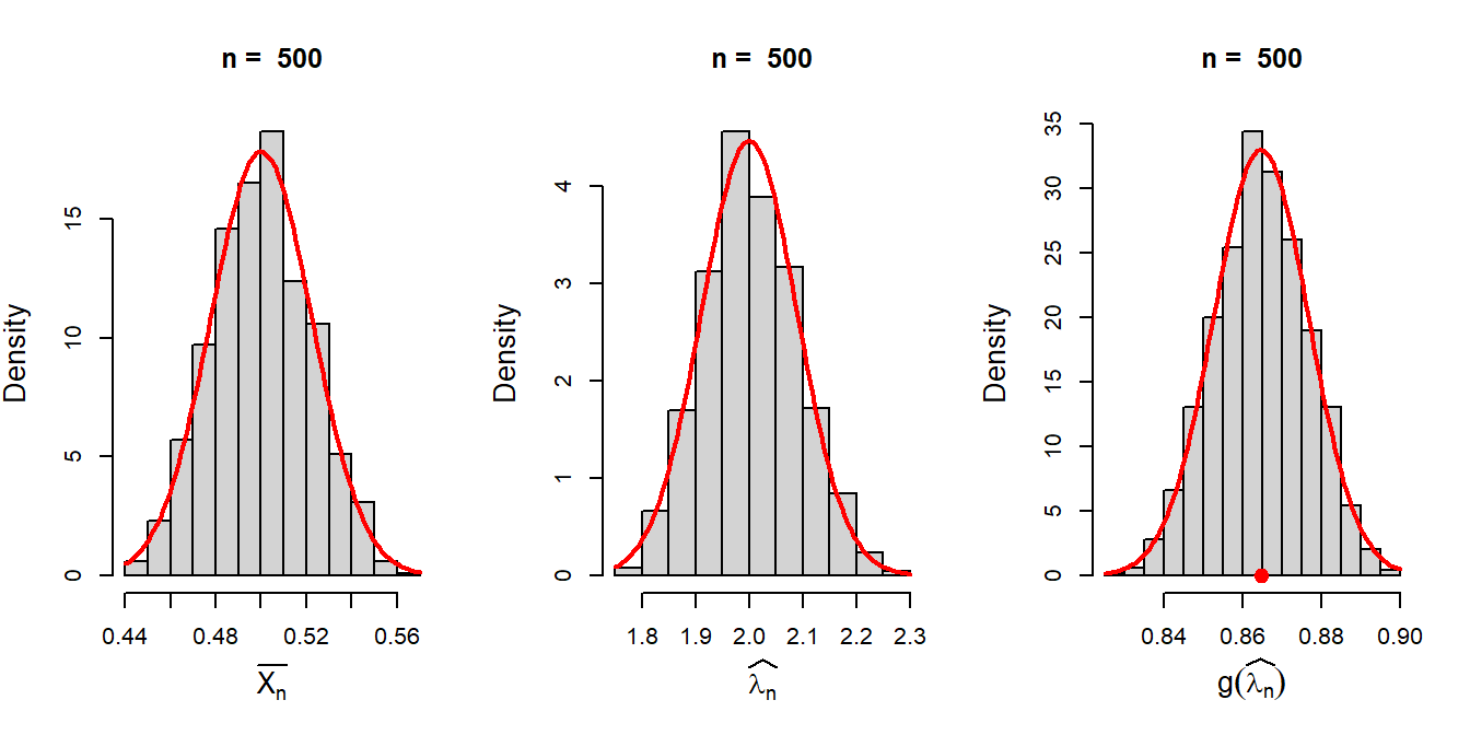
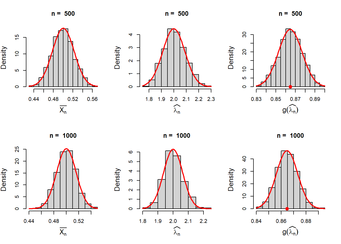
The figure clearly suggested as the sample size \(n\) increases, the sampling distributions of the MLE and the function of MLE are well approximated by the normal distribution. Therefore, if we can compute the mean and variance of the estimators at least for large \(n\), we can get the normal approximation of these histograms.
8.3.5 Normal approximation of \(\widehat{\lambda_n}\)
Consider \(\widehat{\lambda_n} = g\left(\overline{X_n}\right) = \frac{1}{\overline{X_n}}\). Taking Taylor expansion of first order about the expected value of \(\overline{X_n} = \frac{1}{\lambda}\) \(\lambda\), we get \[g\left(\overline{X_n}\right)\approx g\left(\frac{1}{\lambda}\right) + \left(\overline{X_n} - \frac{1}{\lambda}\right)g'\left(\frac{1}{\lambda}\right).\] Since \(\mbox{E}\left(\overline{X_n}\right)=\frac{1}{\lambda}\), we get \[\mbox{E}\left(\widehat{\lambda_n}\right)= \mbox{E}\left(\frac{1}{\overline{X_n}}\right) \approx g\left(\frac{1}{\lambda}\right) = \lambda.\] Therefore, the MLE \(\widehat{\lambda_n}\) is asymptotically unbiased estimator of \(\lambda\). To compute the variance, we observe that \[Var\left(\widehat{\lambda_n}\right)\approx \mbox{E}\left(\widehat{\lambda_n}-\lambda\right)^2 \approx \mbox{E}\left(\overline{X_n}-\frac{1}{\lambda}\right)^2\left(g'\left(\frac{1}{\lambda}\right)\right)^2 = \frac{\lambda^4}{\lambda^2 n}=\frac{\lambda^2}{n}.\] Therefore, we can overlay a normal distribution on the simulated histograms approximating the sampling distribution of \(\widehat{\lambda_n}\) and check whether \[\widehat{\lambda_n} \overset{a}{\sim} \mathcal{N}\left(\lambda, \frac{\lambda^2}{n}\right).\]
In the next phase, we can approximate the mean and variance of \(\widehat{\psi_n} = g\left(\widehat{\lambda_n}\right)\), (say), where \(g(x)=1-e^{-x}\). Considering the first order Taylor’s approximation of \(g\left(\widehat{\lambda_n}\right)\) about the expected value of \(\widehat{\lambda_n}\), which is approximately equal to \(\lambda\) for large \(n\), we obtain:
\[g\left(\widehat{\lambda_n}\right) \approx g(\lambda)+\left(\widehat{\lambda_n}-\lambda\right)g'(\lambda)\] As \(n\to \infty\), \(\mbox{E}\left(\widehat{\psi_n}\right)=\mbox{E}\left[g\left(\widehat{\lambda_n}\right)\right] \approx g(\lambda) = 1-e^{-\lambda}=\psi\), therefore, \(\widehat{\psi_n}\) is an asymptotically unbiased estimator of \(\psi\). The approximate variance of \(\widehat{\psi_n}\), for large \(n\) is obtained as \[Var\left(\widehat{\psi_n}\right)\approx \mbox{E}\left(\widehat{\psi_n}-\psi\right)^2 = \mbox{E}\left[g\left(\widehat{\lambda_n}\right)-g(\lambda)\right]^2 \approx \mbox{E}\left(\widehat{\lambda_n}-\lambda\right)^2\left(g'(\lambda)\right)^2.\] This gives \(Var\left(\widehat{\psi_n}\right) \approx \frac{\lambda^2 e^{-2\lambda}}{n}\). Therefore, we can claim that \[\widehat{\psi_n} = 1- e^{-\widehat{\lambda_n}}\overset{a}{\sim} \mathcal{N}\left(1-e^{-\lambda}, \frac{\lambda^2 e^{-2\lambda}}{n}\right).\]
8.3.6 Visualization for different choices of \(n\)
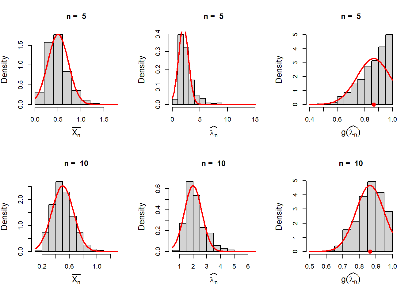
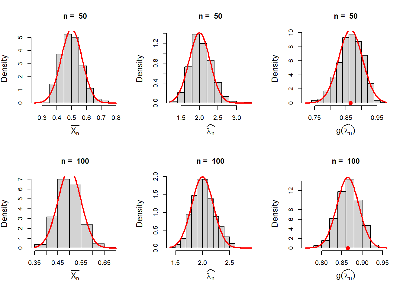
In the above approximations, we have approximated the sampling distribution of \(\overline{X_n}\), \(\widehat{\lambda_n}\) and \(\widehat{\psi_n} = g(\widehat{\lambda_n})=1-e^{-\widehat{\lambda_n}}\) for a fixed value of \(n\) using the normal distribution. In the following codes, we visualize the sampling distribution for different choices of \(n\). The histograms are overlaid with the normal distribution with the mean and variance computed by the Delta method.
n_vals = c(5, 10, 50, 100, 500, 1000)
par(mfrow = c(2,3))
M = 1000
lambda = 2
for(n in n_vals){
  sample_means = numeric(length = M)
  lambda_hat = numeric(length = M)
  psi_hat = numeric(length = M)
  for (i in 1:M) {
    x = rexp(n = n, rate = lambda)
    sample_means[i] = mean(x)
    lambda_hat[i] = 1/mean(x)
    psi_hat[i] = 1 - exp(-lambda_hat[i])
  }
  hist(sample_means, probability = TRUE,
       main = paste("n = ", n), xlab = expression(bar(X[n])), cex.lab = 1.3)
  curve(dnorm(x, mean = 1/lambda, sd = 1/sqrt(lambda^2*n)),
        add = TRUE, col = "red", lwd = 2)

  hist(lambda_hat, probability = TRUE,
       main = paste("n = ", n), xlab = expression(widehat(lambda[n])), cex.lab = 1.3)
  curve(dnorm(x, mean = lambda, sd = sqrt(lambda^2/n)),
        add = TRUE, col = "red", lwd = 2)

  hist(psi_hat, probability = TRUE,
       main = paste("n = ", n), xlab = expression(g(widehat(lambda[n]))), cex.lab = 1.3)
  points(psi, 0, pch = 19, col = "red",
         cex = 1.4)
  curve(dnorm(x, mean = psi, sd = sqrt(lambda^2*exp(-2*lambda)/n)),
        add = TRUE, col = "red", lwd = 2)
}
Invariance property of MLE
Suppose \(X_1,\ldots,X_n\) be a random sample from the population PDF (PMF) \(f(x|\theta)\). If \(\widehat{\theta_n}\) be the MLE of \(\theta\), then for any function \(g(\theta)\), the MLE of \(g(\theta)\) is \(g\left(\widehat{\theta_n}\right)\).
8.4 Approximation of the Risk function
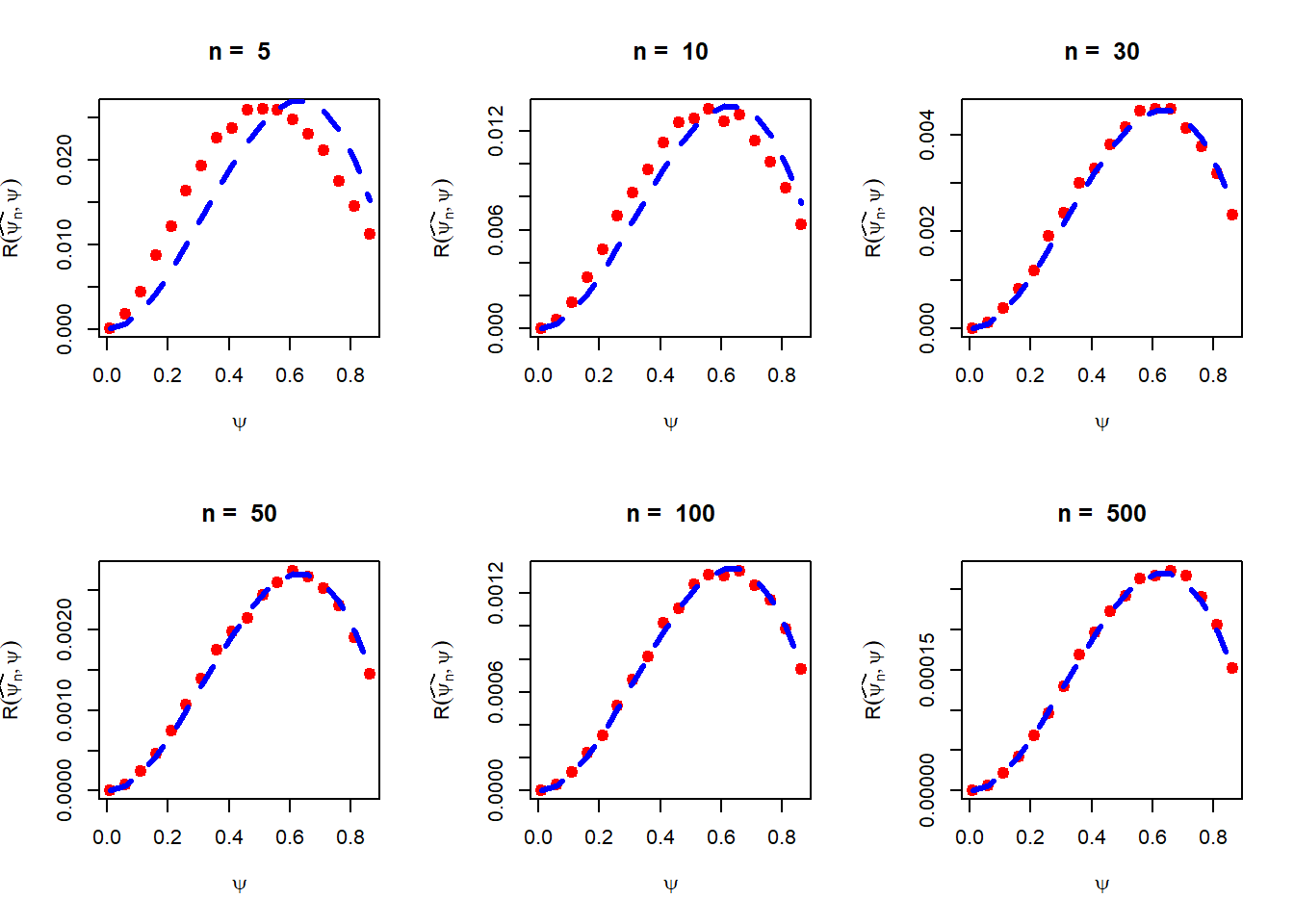
In the language of risk function, we can write that for large \(n\), \[\mathcal{R}\left(\widehat{\lambda_n},\lambda\right)=\mbox{E}\left(\widehat{\lambda_n}-\lambda\right)^2 \approx \frac{\lambda^2}{n}.\] However, for the estimator \(\widehat{\psi_n}\), we have computed the risk as a function of \(\lambda\) only. By expressing \(\lambda\) in terms of \(\psi\) (it is a monotone transformation from \(\lambda \to \psi\)) as \(\lambda = -\log(1-\psi)\), we obtain the approximate risk function as \[\mathcal{R}\left(\widehat{\psi_n},\psi\right) \approx \frac{(-(1-\psi)\log(1-\psi))^2}{n}, \mbox{ for large }n, \psi\in(0,1).\]
The verification of the above expression can be performed by computer simulation. Instead of discretizing the range of \(\lambda\), discretize the possible parameter space corresponds to \(\psi\in(0,1)\).
par(mfrow = c(2,3))
n_vals = c(5, 10, 30, 50, 100, 500)
M = 5000
psi_vals = seq(0.01, 0.9, by = 0.05)
for(n in n_vals){
  risk_psi_hat = numeric(length = length(psi_vals))
  for(i in 1:length(psi_vals)){
    psi = psi_vals[i]                        # true probability
    lambda = -log(1-psi)                     # rate for exponential
    loss_psi_hat = numeric(length = M)
    for(j in 1:M){
      x = rexp(n = n, rate = lambda)
      psi_hat = 1-exp(-1/mean(x))
      loss_psi_hat[j] = (psi_hat-psi)^2
    }
    risk_psi_hat[i] = mean(loss_psi_hat)
  }
  plot(psi_vals, risk_psi_hat, col = "red", xlab = expression(psi),
       ylab = expression(R(widehat(psi[n]),psi)),
       main = paste("n = ", n), pch = 19, cex = 1.3)
  lines(psi_vals, (-(1-psi_vals)*log(1-psi_vals))^2/n,
        col = "blue", lwd = 3, lty = 2)
}
Delta Method
Let \(W_n\) be a sequence of random variables that satisfies \[\sqrt{n}\left(W_n-\theta\right)\overset{a}{\sim}\mathcal{N}(0,\sigma^2)\] in distribution. For a given function \(g(\cdot)\) and a specific value of \(\theta\in \Theta\), suppose that \(g'(\theta)\) exists and \(g'(\theta)\ne 0\). Then \[\sqrt{n}\left[g\left(W_n\right)-g(\theta)\right] \overset{a}{\sim}\mathcal{N}\left(0, \sigma^2\left[g'(\theta)\right]^2\right),\] in distribution.
The basic idea is that as the sample size increases, the function of asymptotically normally distributed random variables can also be approximated by the normal distribution mean and variance can be easily computed by using the first order Taylor’s polynomial approximation.
Comparing Risk Functions
Suppose in the same problem of estimating \(\psi = \mbox{P}(X\ge 1)\), another alternative estimator \[\widehat{\xi_n}=\frac{1}{n}\sum_{i=1}^nI(X_i\ge 1)\] is suggested, where the quantity \(I(X\ge 1)\) is defined as \[I(X\ge 1) = \begin{cases} 1, X\ge 1 \\ 0, X<1 \end{cases}.\] Therefore, \(\widehat{\xi_n}\) basically the proportion of observations which are greater than or equal to \(1\). It is easier to check that \(\mbox{E}\left(\widehat{\xi_n}\right) = \psi\) and \(Var\left(\widehat{\xi_n}\right) = \frac{\psi(1-\psi)}{n}\). Using computer simulation, simulate the risk function \(\mathcal{R}\left(\widehat{\xi_n},\psi\right)\) and compare it with \(\mathcal{R}\left(\widehat{\psi_n},\psi\right)\) at different values of \(\psi \in(0,1)\) for different sample sizes \(n\). Write your conclusion in simple English language.
8.5 Multi-parameter optimization
In the previous sections, we have learnt that how one can obtain the sampling distribution of the MLE and also tested whether the MLE converges in probability to the true parameter value by using computer simulations. Many real life problems are modeled by probability distributions which is parameterized by more than one parameters, for example, \(\mathcal{N}(\mu, \sigma^2)\), \(\mathcal{B}(a,b)\), \(\mathcal{G}(a,b)\), etc. In this section, we consider the computation of the MLE for multiparameter probability distributions.
Suppose that we have a random sample \((X_1,X_2,\ldots,X_n)\) of size \(n\) from the normal distribution with parameters \(\mu\) and \(\sigma^2\). Our goal is to obtain the Maximum Likelihood Estimators of \(\mu\) and \(\sigma^2\) based on the sample observations and study properties of these estimators. The parameter space is \[\Theta = \left\{\left(\mu,\sigma^2\right)\colon -\infty<\mu<\infty, 0<\sigma<\infty\right\}\]
n = 30
mu = 3
sigma2 = 1.5
x = rnorm(n = n, mean = mu, sd = sqrt(sigma2))
hist(x, probability = TRUE)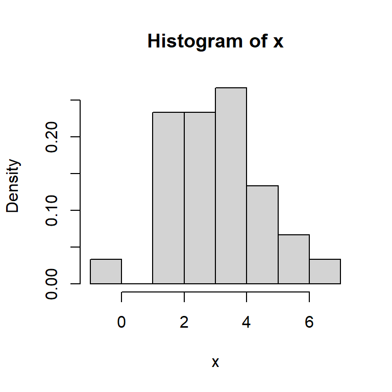
8.5.1 Likelihood function
If \((x_1,x_2,\ldots,x_n)\) be a fixed observed sample of size \(n\), then the likelihood function is given by \[\mathcal{L}(\mu,\sigma^2)=\left(2\pi\sigma^2\right)^{-\frac{n}{2}}e^{-\frac{1}{2\sigma^2}\sum_{i=1}^n\left(x_i-\mu\right)^2}, -\infty<\mu<\infty, 0<\sigma<\infty.\] The log-likelihood function is given by \[l\left(\mu,\sigma^2\right)=\log \mathcal{L}(\mu,\sigma^2)=-\frac{n}{2}\log(2\pi\sigma^2)-\frac{1}{2\sigma^2}\sum_{i=1}^n\left(x_i - \mu\right)^2.\] - Compute \(\frac{\partial l}{\partial \mu}\) and \(\frac{\partial l}{\partial \sigma^2}\) and set them equal to zero. - Solve the above system simultaneously and obtain the critical points \(\mu^*\) and \(\sigma^{2^*}\). - Show the the the following matrix \[H = \begin{bmatrix} \frac{\partial^2 l}{\partial \mu^2} & \frac{\partial^2 l}{\partial \mu \partial \sigma^2} \\ \frac{\partial^2 l}{\partial \mu \partial \sigma^2} & \frac{\partial^2 l}{\partial (\sigma^2)^2} \end{bmatrix}\] is negative definite when the partial derivatives are evaluated at \(\left(\mu^*, \sigma^{2^*}\right)\). This can be checked by ensuring the following two conditions: \[H_{11}<0,~~\mbox{and}~~~\det(H) = H_{11}H_{22} - \left(H_{12}\right)^2>0.\]
In the following, we plot the likelihood function and the log-likelihood function as a function of the parameters \(\mu\) and \(\sigma^2\).
Likelihood = function(mu, sigma2){
  (1/(sigma2*2*pi)^(n/2))*exp(-sum(x-mu)^2/(2*sigma2))
}

LogLikelihood = function(mu, sigma2){
  log(Likelihood(mu = mu, sigma2 = sigma2) + 0.5)
}

mu_vals = seq(2, 4, by = 0.1)
sigma2_vals = seq(1, 1.5, by = 0.1)

Lik_vals = matrix(data = NA, nrow = length(mu_vals),
                  ncol = length(sigma2_vals))
LogLik_vals = matrix(data = NA, nrow = length(mu_vals),
                  ncol = length(sigma2_vals))
for(i in 1:length(mu_vals)){
  for(j in 1:length(sigma2_vals)){
    Lik_vals[i,j] = Likelihood(mu = mu_vals[i],
                               sigma2 = sigma2_vals[j])
    LogLik_vals[i,j] = LogLikelihood(mu = mu_vals[i],
                               sigma2 = sigma2_vals[j])
  }
}
par(mfrow = c(1,2))
persp(mu_vals, sigma2_vals, Lik_vals, theta = 60, col = "yellow", )
persp(mu_vals, sigma2_vals, LogLik_vals, theta = 60, col = "yellow")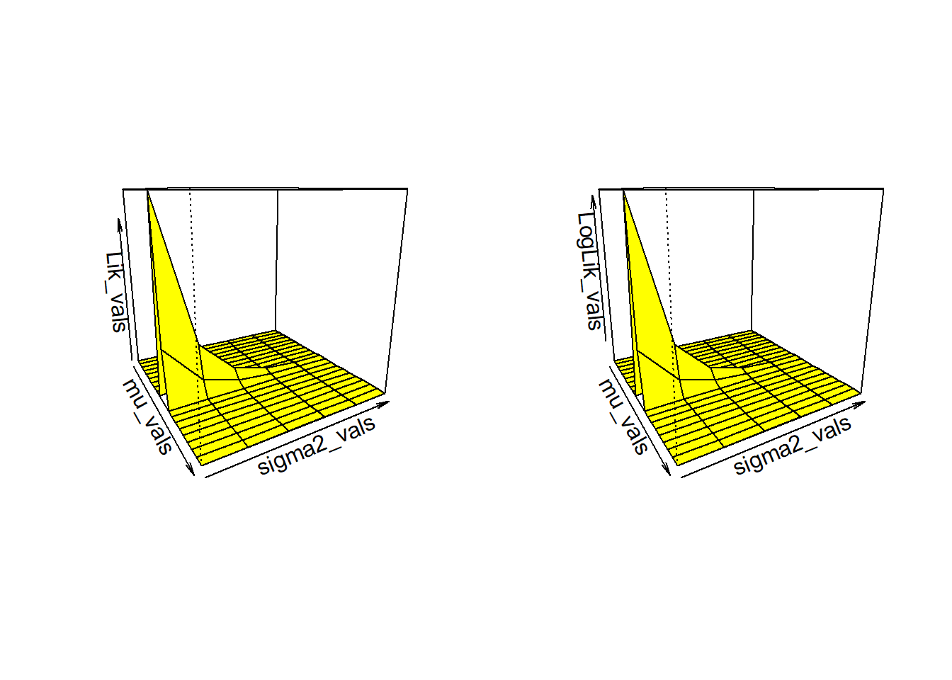
From the computation, we observed that the MLE of the \(\mu\) and \(\sigma^2\) are given by
\[\widehat{\mu_n} = \overline{X_n},~~~~\widehat{\sigma^2_n} = \frac{1}{n}\sum_{i=1}^n \left(X_i - \overline{X_n}\right)^2\] Given an estimators, the following questions immediately appear, such as (a) are these estimators unbiased? (b) are these estimators consistent, (c) are these estimators are the best choices under some given loss function? We shall not address all these questions here only, but, certainly show how we basic properties of these estimators can be checked and when feasible, we shall also compute the exact sampling distribution of these estimators.
At the first step, let us check whether as the sample size increases, the MLEs converge to the true parameter values. Mathematically, whether the following statements true: \[\overline{X_n} \overset{P}{\to}\mu,~~~~\mbox{and}~~~~\widehat{\sigma_n^2} \overset{P}{\to} \sigma^2.\] The following simulation will help us to understand whether the above statements are true.
- Fix sample size \(n\in\{2,3,\ldots,1000\}\).
- Fix \(\mu = \mu_0\) and \(\sigma^2=\sigma_0^2\).
- For each \(n\)
- Simulate \(X_1, X_2, \ldots, X_n \sim \mathcal{N}\left(\mu_0, \sigma_0^2\right)\).
- Compute \(\overline{X_n}\) and \(\widehat{\sigma_n^2}\)
- Plot the pairs \(\left(n,\overline{X_n}\right)\) and \(\left(n, \widehat{\sigma_n^2}\right)\)
- Add a horizontal straight line to the plots at \(\mu_0\) and \(\sigma_0^2\), respectively.
n_vals = 2:1000
mu_hat = numeric(length = length(n_vals))
sigma2_hat = numeric(length = length(n_vals))
for(i in 1:length(n_vals)){
  n = n_vals[i]
  x = rnorm(n = n, mean = mu, sd = sqrt(sigma2))
  mu_hat[i] = mean(x)
  sigma2_hat[i] = (1/n)*sum((x-mean(x))^2)
}
par(mfrow = c(1,2))
plot(n_vals, mu_hat, col = "grey", lwd = 2,
     xlab = "sample size (n)", ylab = expression(widehat(mu[n])))
abline(h = mu, col = "blue", lwd = 3, lty = 2)
plot(n_vals, sigma2_hat, col = "grey", lwd = 2,
     xlab = "sample size (n)", ylab = expression(widehat(sigma[n]^2)))
abline(h = sigma2, col = "blue", lwd = 3, lty = 2)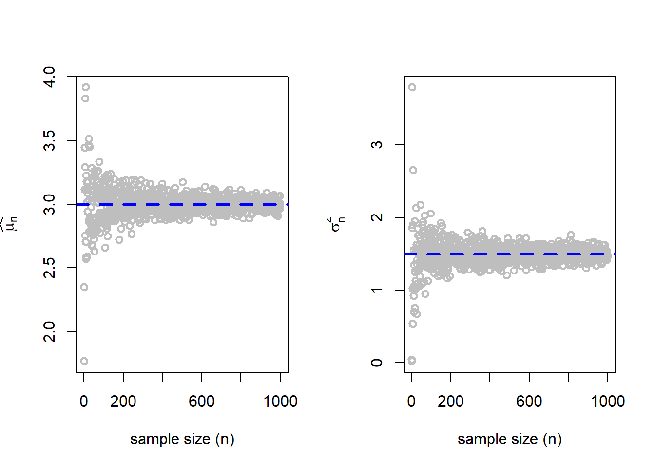
To quantify the uncertainty associated with the MLE, we can either obtain the exact sampling distributions of \(\overline{X_n}\) and \(\widehat{\sigma_n^2}\), or we can approximate the standard error of these estimators at different true values by computer simulations by fixing \(n\). Let us fix the value of \(n\) and simulate \(M=1000\) realizations from the sampling distributions of the MLEs and visualize their distribution through histograms.
n = 10                                  # sample size
M = 1000                                # number of replications
mu_hat = numeric(length = M)
sigma2_hat = numeric(length = M)
for(i in 1:M){
  x = rnorm(n = n, mean = mu, sd = sqrt(sigma2))
  mu_hat[i] = mean(x)
  sigma2_hat[i] = (1/n)*sum((x-mean(x))^2)
}
par(mfrow = c(1,2))
hist(mu_hat, probability = TRUE, main = paste("n = ", n),
     xlab = expression(widehat(mu[n])), breaks = 30)
curve(dnorm(x, mean = mu, sd = sqrt(sigma2/n)),
      add = TRUE, col = "red", lwd = 2)
hist(sigma2_hat, probability = TRUE, main = paste("n = ", n),
     xlab = expression(widehat(sigma[n]^2)), breaks = 30)
dist_sigma2_hat = function(x){

  num = exp(-n*x/(2*sigma2))*(n*x/sigma2)^((n-1)/2-1)*n*(x>0)
  den = gamma((n-1)/2)*2^((n-1)/2)*sigma2
  return(num/den)
}
curve(dist_sigma2_hat(x), add = TRUE, col = "red", lwd = 2)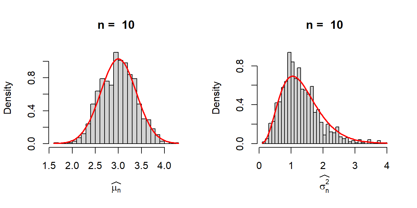
In the classroom, Sangeeta has pointed out that sample mean would in fact follow the normal distribution due to the Central Limit Theorem (\(n\) large). The statement is indeed true. However, since the sampling has been carried out from the normal distribution, the sample mean has an exact normal distribution with mean \(\mu\) and variance \(\frac{\sigma^2}{n}\) for every \(n\) (not only for large \(n\)), which can be proved using the MGF technique, shown below: \[M_{\overline{X_n}}(t) = \cdots \mbox{ fill the gap }\cdots = e^{\mu t + \frac{1}{2}\left(\frac{\sigma^2}{n}\right)t}, -\infty<t<\infty.\]
While for the sample mean, the computation is apparently straightforward application of the MGF. For the the MLE of \(\sigma^2\), a slightly lengthier calculations is required. In the following subsection, we list main results related to the sampling from the normally distributed population.
Sampling from the normal distribution
Let \(X_1, X_2,\ldots,X_n\) be a random sample of size \(n\) from the \(\mathcal{N}(\mu, \sigma^2)\) population distribution. Then
- \(\overline{X_n}\) and \(S_n^2\) are independent random variables.
- \(\overline{X_n}\) has a \(\mathcal{N}\left(\mu, \frac{\sigma^2}{n}\right)\) distribution.
- \(\frac{(n-1)S_n^2}{\sigma^2}\) has a \(\chi_{n-1}^2\) distribution with \(n-1\) degrees of freedom.
Reader is encouraged to see the proofs in (Casella and Berger 2002) and (Rohatgi and Saleh 2000). I encourage to see both the proofs as they used two different approaches. Casella and Berger (2002) used the transformation formula to explicitly derive the joint distribution of \(\overline{X_n}\) and \(S_n^2\), whereas Rohatgi and Saleh (2000) elegantly used the joint moment generating function to prove the above results.
Considering \(U_n = \frac{(n-1)S_n^2}{\sigma^2}\sim \chi_{n-1}^2\), the sampling distribution of the MLE \(V_n = \widehat{\sigma_n^2} = \frac{\sigma^2}{n}\times U_n\) can be easily obtained. The CDF of \(V_n\) is obtained as
\[F_{V_n}(v)=\mbox{P}(V_n \le v) = \mbox{P}\left(U_n\le \frac{nv}{\sigma^2}\right).\] Therefore, \[f_{V_n}(v) = \frac{d}{dv}F_{V_n}(v)=f_{U_n}\left(\frac{nv}{\sigma^2}\right)\cdot\frac{n}{\sigma^2}, 0<v<\infty.\] For every \(n\), the sampling distribution of the MLE of \(\sigma^2\), \(\widehat{\sigma_n^2}\) is given by: \[f_{\widehat{\sigma_n^2}}(v)=\frac{e^{-\frac{nv}{2\sigma^2}}\left(\frac{nv}{\sigma^2}\right)^{\frac{n-1}{2}-1}}{\Gamma\left(\frac{n-1}{2}\right)2^{\frac{n-1}{2}}}\cdot \frac{n}{\sigma^2}, 0<v<\infty.\]
mu = 3
sigma2 = 1.5
n_vals = c(3,5,10,50,100, 200)
M = 1000
par(mfrow = c(2,3))
for(n in n_vals){
  mu_hat = numeric(M)
  sigma2_hat = numeric(M)
  for(i in 1:M){
    x = rnorm(n = n, mean = mu, sd = sqrt(sigma2))
    sigma2_hat[i] = (1/n)*sum((x-mean(x))^2)
  }
  hist(sigma2_hat, probability = TRUE, main = paste("n = ", n), xlab = expression(widehat(sigma[n]^2)))
  curve(dist_sigma2_hat(x), add = TRUE, col = "red", lwd = 2)
  points(sigma2, 0, pch = 19, col = "red", cex = 1.5)
  points(mean(sigma2_hat), 0, col = "blue", lwd = 3,
         cex = 2)
}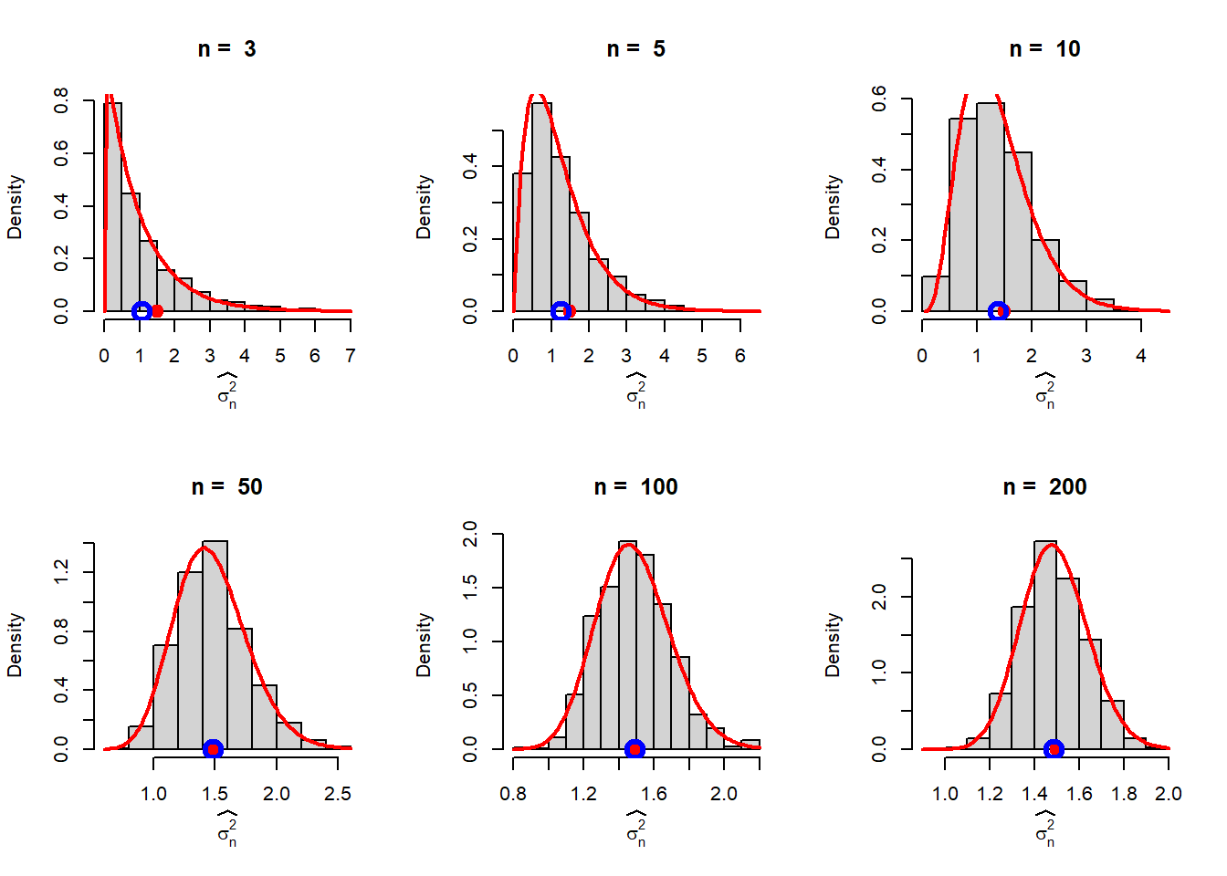
By performing the above exercises for different choices of \(n\), we observed that the this sampling distribution is valid for every \(n\). However, as \(n\) increases, the shapes of the sampling distributions eventually tends to the normal distribution. We need to give some reasoning for this which is intuitively appealing.
Let us explore the connections between \(U_n = \frac{n-1}{n}S_n^2\) and \(V_n = \widehat{\sigma_n}^2 = \frac{\sigma^2}{n}\times U_n\) and their approximation by the normal distribution for large \(n\). Suppose that we are given the fact that for every \(n\), \(U_n \sim \chi^2_{n-1}\) distribution. The PDF of \(V_n\) has been obtained by using the transformation formula. The shapes of the PDF of \(V_n\) in fact shows a normally distributed behavior for large \(n\) values. Since, the chi squared distribution belongs to the \(\mathcal{G}(\cdot,\cdot)\) family, \(V_n\) is a constant multiple of a \(\mathcal{G}\left(\alpha = \frac{n-1}{2},\beta = 2\right)\equiv\chi_{n-1}^2\).
Therefore, if we can show that for large \(n\), \(\chi_n^2\) distribution can be well approximated by the normal distribution, we are done. In the following we show that for large \(n\), \(\chi_n^2\) PDF is well approximated by the normal distribution with mean \(n\) and variance \(2n\). We investigate the MGF of \(\frac{X-n}{\sqrt{2n}}\) and see that it is approximately \(e^{\frac{t^2}{3}}\) for large \(n\).
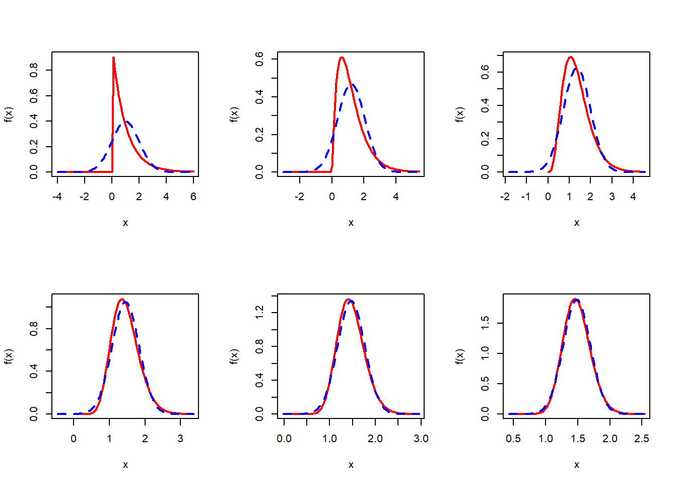
\[\log\left[M_{\frac{X-n}{\sqrt{2n}}}(t)\right]=-\sqrt{\frac{n}{2}}t+\frac{n}{2}\log\left(1-\frac{t}{\sqrt{\frac{n}{2}}}\right)=\frac{t^2}{2}+ \mathcal{O}\left(\frac{1}{n^{3/2}}\right).\] Therefore, \[\frac{X-n}{\sqrt{2n}} \overset{a}{\sim}\mathcal{N}(0,1)\implies X \overset{a}{\sim}\mathcal{N}\left(n, 2n\right).\] Therefore \(U_n \sim \mathcal{N}(n-1, 2(n-1))\) for large \(n\). Hence, \[V_n = \widehat{\sigma_n^2} = \frac{\sigma^2}{n}\times U_n\overset{n \mbox{ large}}{\sim} \mathcal{N}\left(\frac{(n-1)\sigma^2}{n},\frac{2(n-1)\sigma^4}{n^2}\right).\] In the following, R Codes, the exact sampling distribution of \(\widehat{\sigma_n^2}\) and the normal approximation is shown graphically and the approximations are remarkable accurate for large \(n\) values.
n_vals = c(3,5,10,30,50,100)
par(mfrow = c(2,3))
for(n in n_vals){
  lower_lim = sigma2*(n-1)/n- 5*sqrt(sigma2^2*2*(n-1)/n^2)
  upper_lim = sigma2*(n-1)/n+ 5*sqrt(sigma2^2*2*(n-1)/n^2)

  curve(dist_sigma2_hat(x), col = "red", lwd = 2, lower_lim, upper_lim, ylab = "f(x)")

  curve(dnorm(x,mean = sigma2*(n-1)/n, sd = sqrt(sigma2^2*2*(n-1)/n^2)),
        add = TRUE, lty = 2, col = "blue", lwd = 2)
}
8.6 Connection between the Hessian and Fisher Information
In the examples discussed above, the MLEs have always appeared to be approximately normal at least for large \(n\) and centered about the true value of the parameter. However, we did not explore yet the computation of the variance of the MLEs. In fact, some analytical computation for the variance can be carried out and established as well by computer simulation. We consider some definition first.
Score Function and Fisher Information
If \(\mathbf{X}=(X_1,X_2,\ldots,X_n)\) be a random sample of size \(n\) from the PDF (PMF) \(f(x|\theta)\), \(\theta\in \Theta\).
The Score function is defined as \[S(\mathbf{X};\theta) = \frac{\partial \log f\left(\mathbf{X}|\theta\right)}{\partial \theta}.\] It can be easily shown that \[\mbox{E}_{\theta}\left[S(\mathbf{X};\theta)\right]=0.\]
The Fisher Information is defined as \[I_n(\theta)=Var_{\theta}\left(\sum_{i=1}^n S\left(X_i;\theta\right)\right)=\sum_{i=1}^n Var_{\theta}\left(S\left(X_i;\theta\right)\right)=\sum_{i=1}^n\mbox{E}_{\theta}\left(S\left(X_i;\theta\right)\right)^2.\] The Fisher Information can also be expressed as \[I_n(\theta)= -\mbox{E}_{\theta}\left(\frac{\partial^2\log f\left(\mathbf{X}|\theta\right)}{\partial \theta^2}\right)=-\int_{\mathbb{R}^n}\left(\frac{\partial^2\log f\left(\mathbf{x}|\theta\right)}{\partial \theta^2}\right)f(\mathbf{x|\theta})d\mathbf{x}.\]
A natural question arises, how to interpret the expectation of the score function. Here is an interpretation in terms of simulation.
- Fix parameter \(\theta = \theta_0\)
- Fix the sample size \(n\)
- Fix the number of replications \(M\)
- For each \(m\in \{1,2,\ldots,M\}\)
- Simulate \(\mathbf{X}=(X_1,\ldots,X_n)\sim f(x|\theta_0)\).
- Compute \(S(\mathbf{X};\theta_0) = S_m\) (say)
- \(\frac{1}{M}\sum_{m=1}^M S_m \overset{M\to \infty}{\approx} \mbox{E}\left(S\left(\mathbf{X};\theta_0\right)\right)=0\)
8.6.1 Visualization of the Score function
In the following, we visualize the score function for the Poisson distribution. We simulate multiple sets of random sample of size \(n=10\) from the \(\mbox{Poisson}(\lambda_0)\) distribution and plot the score function as a function of \(\lambda\).
par(mfrow = c(1,1))
lambda_0 = 3                     # true value
n = 10                           # sample size
x = rpois(n = n, lambda = lambda_0)
score_poisson = function(lambda){
  -n + sum(x)/lambda
}
lambda_vals = seq(1, 5, by = 0.01)
score_vals = numeric(length = length(lambda_vals))
for(i in 1:length(lambda_vals)){
  score_vals[i] = score_poisson(lambda = lambda_vals[i])
}
plot(lambda_vals, score_vals, type = "l",
     col = "grey", lwd = 2, xlab = expression(lambda),
     ylab = expression(S(bold(X),lambda)))
points(lambda_0, 0, pch = 19, col = "red", cex = 1.4)
abline(h = 0, lwd = 2, col = "blue", lty = 2)
points(mean(x), 0, col = "blue", cex = 2, lwd = 2,
       pch = 19)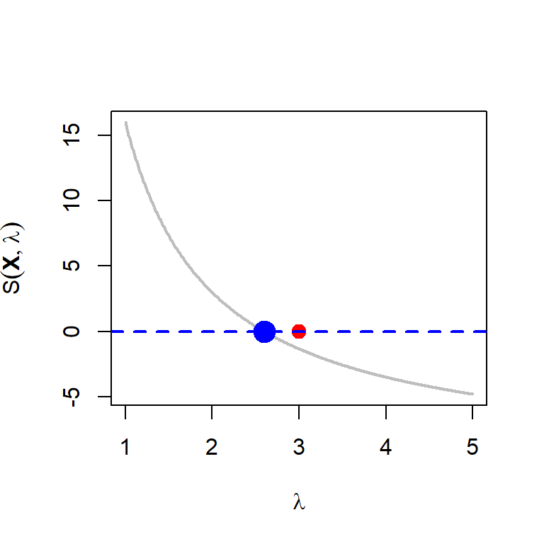
Let us repeat the above process and plot the score functions in a single plot.
n = 10
M = 50
lambda_0 = 3
for (i in 1:M) {
  data = rpois(n = n, lambda = lambda_0)
  if(i == 1)
    curve(-n+sum(data)/x, 1, 5, col = "grey", lwd = 2,
          xlab = expression(lambda), ylab = expression(S(bold(X),lambda)))
  else
    curve(-n+sum(data)/x, add= TRUE, col = "grey",
          lwd = 2)
  points(mean(data), 0, col = "blue", cex = 1, lwd = 2,
       pch = 19)
}
points(lambda_0, 0, pch = 19, col = "red", cex = 1.4)
abline(h = 0, lwd = 2, col = "blue", lty = 2)
abline(v = lambda_0, col = "magenta", lty = 2, lwd = 3)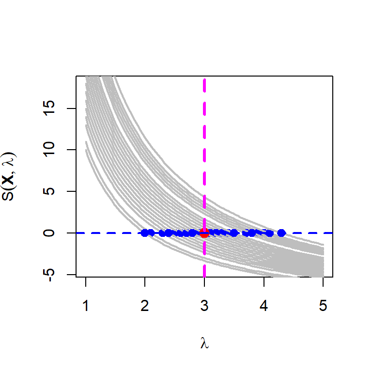
Let us do the same experiment for the Cauchy distribution whose score function is given by \[S(\mathbf{X};\mu) = 2\sum_{i=1}^n \frac{(x_i - \mu)}{\left[1+(x_i-\mu)^2\right]}\]
par(mfrow = c(1,1))
mu_0 = 3           # true value
n = 10
x = rcauchy(n = n, location = mu_0)
score_cauchy = function(mu){
  2*sum((x-mu)/(1+(x-mu)^2))
}
mu_vals = seq(1, 5, by = 0.01)
score_vals = numeric(length = length(mu_vals))
for(i in 1:length(mu_vals)){
  score_vals[i] = score_cauchy(mu = mu_vals[i])
}
plot(mu_vals, score_vals, type = "l",
     col = "grey", lwd = 2, xlab = expression(mu),
     ylab = expression(S(bold(X),mu)))
points(mu_0, 0, pch = 19, col = "red", cex = 1.4)
abline(h = 0, lwd = 2, col = "blue", lty = 2)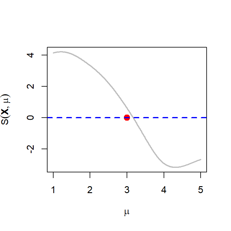
8.6.2 Asymptotic distribution of the MLE
Under certain regularity conditions for the studied population distribution \(f(x|\theta)\), if \(\widehat{\theta_n}\) be the MLE of \(\theta\) and \(I_{n}(\theta)\) be the Fisher Information. Then \(\mbox{SE}\left(\widehat{\theta_n}\right) = \sqrt{Var\left(\widehat{\theta_n}\right)} \approx \sqrt{\frac{1}{I_n(\theta)}}\). In addition \[\frac{\widehat{\theta_n}-\theta}{\mbox{SE}\left(\widehat{\theta_n}\right)} \to \mathcal{N}(0,1),~~\mbox{in distribution}.\]
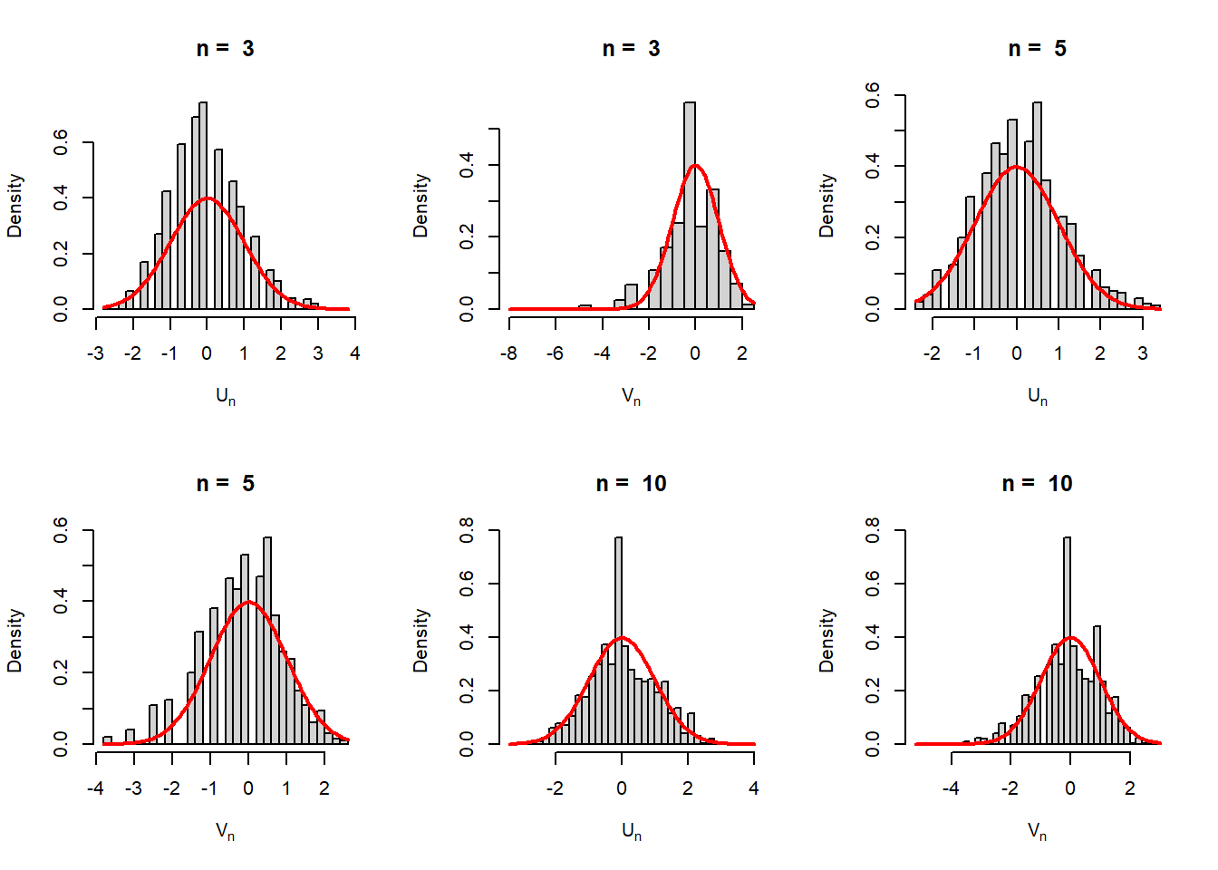
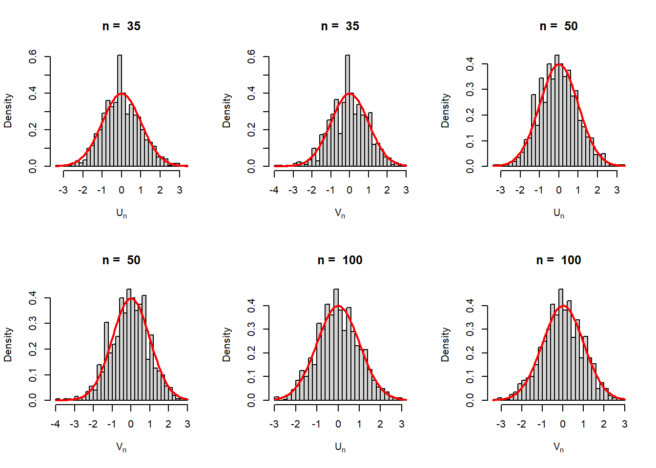
In addition, \(\widehat{\mbox{SE}}\left(\widehat{\theta_n}\right) = \sqrt{\widehat{Var}\left(\widehat{\theta_n}\right)} \approx \sqrt{I_n\left(\widehat{\theta_n}\right)^{-1}}\) and \[\frac{\widehat{\theta_n}-\theta}{\widehat{\mbox{SE}}\left(\widehat{\theta_n}\right)} \to \mathcal{N}(0,1),~~\mbox{in distribution}.\] In the following simulation experiment, we verify the above results for the Poisson distribution. The MLE for the parameter \(\lambda\) is \(\widehat{\lambda_n}=\overline{X_n}\). \(\mbox{SE}\left(\widehat{\lambda_n}\right) = \sqrt{\frac{\lambda}{n}}\) and \(\widehat{\mbox{SE}}\left(\widehat{\lambda_n}\right) = \sqrt{\frac{\widehat{\lambda_n}}{n}}=\sqrt{\frac{\overline{X_n}}{n}}\).
par(mfrow = c(2,3))
lambda_0 = 3
M = 1000
n_vals = c(3, 5, 10, 35, 50, 100)
for(n in n_vals){
  U = numeric(length = M)
  V = numeric(length = M)
  for(i in 1:M){
    x = rpois(n = n, lambda = lambda_0)
    U[i] = (mean(x)-lambda_0)/(sqrt(lambda_0/n))
    V[i] = (mean(x)-lambda_0)/(sqrt(mean(x)/n))
  }
  hist(U, probability = TRUE, main = paste("n = ", n), breaks = 30,
       xlab = expression(U[n]))
  curve(dnorm(x), add = TRUE, col = "red", lwd = 2)
  hist(V, probability = TRUE, main = paste("n = ", n), breaks = 30,
       xlab = expression(V[n]))
  curve(dnorm(x), add = TRUE, col = "red", lwd = 2)
}
8.6.3 Multiparameter setting and Score function
Suppose that \(X_1,X_2,\ldots,X_n\) be a random sample of size \(n\) from the population PDF (PMF) \(f(x|\theta)\) and \(\theta\in \Theta \subseteq \mathbb{R}^p\) and \(p>1\). Let \(\theta = (\theta_1,\ldots,\theta_p)\) and the corresponding MLE is expressed as \[\widehat{\theta_n} = \left(\widehat{\theta_1},\widehat{\theta_2},\ldots,\widehat{\theta_p}\right).\]
MLE is computed by solving the system of \(p\) equations given by \[\frac{\partial l_n(\theta)}{\partial \theta_j}=0, j\in\{1,2,\ldots,p\}\] We define \[H_{jj} = \frac{\partial^2 l_n(\theta)}{\partial \theta_j^2},~~~\mbox{and}~~~~ H_{jk} = \frac{\partial^2 l_n(\theta)}{\partial \theta_j \partial \theta_k}\] for \(i,j\in \{1,2,\ldots,p\}\). Similar to the one variance case, here we will have the Fisher Information Matrix defined as \[I_n(\theta) = \begin{bmatrix} \mbox{E}_{\theta}(H_{11}) & \mbox{E}_{\theta}(H_{12}) & \cdots & \mbox{E}_{\theta}(H_{1p}) \\ \mbox{E}_{\theta}(H_{21})& \mbox{E}_{\theta}(H_{22}) & \cdots & \mbox{E}_{\theta}(H_{2p})\\ \vdots & \vdots & \vdots & \vdots \\ \mbox{E}_{\theta}(H_{p1}) & \mbox{E}_{\theta}(H_{p2}) & \cdots & \mbox{E}_{\theta}(H_{pp})\end{bmatrix}\] When the partial derivatives are evaluated at the MLE \(\widehat{\theta_n}\), then we obtain the \(\texttt{Observed}\) Fisher Information Matrix.
Fisher Information Matrix and Multivariate Normality of MLE
Let \(J_n = I^{-1}_n(\theta)\), the inverse of the expected Fisher Information Matrix. Under appropriate regularity conditions \[\sqrt{n}\left(\widehat{\theta_n}-\theta_{p\times 1}\right) \overset{n\to \infty}{\sim} \mbox{MVN}_p\left(0, J_n(\theta)\right).\] In particular \[\frac{\sqrt{n}\left(\widehat{\theta_j}-\theta_j\right)}{\widehat{\mbox{SE}}(\widehat{\theta_j})}\overset{n\to \infty}{\sim}\mathcal{N}(0,1)\] where \(\widehat{\mbox{SE}}(\widehat{\theta_j})= J_n(j,j)\), the \(j\)th diagonal entry of \(J_n\), evaluated at \(\widehat{\theta}\). Also \[\mbox{Cov}\left(\widehat{\theta_j}, \widehat{\theta_k}\right) \approx J_n(j,k).\]
8.7 The famous regularity conditions
Throughout the discussions in the statistical computing lectures, we have observed only nice things about the MLE of model parameter(s) \(\theta\), two prominent properties are: (a) MLEs are consistent estimators, that means as the sample size goes to infinity, the sampling distribution of the MLEs will be highly concentrated at the true parameter value \(\theta\), or in other words, the limiting distribution of the MLE is degenerate at the true value. In fact, this property is true for any probability density (or mass) functions \(f(x|\theta), \theta \in \Theta\) which belongs to the family satisfying the following four conditions:
- The random sample \(X_1,X_2,\ldots,X_n\) are independent and identically distributed (IID) following \(f(x|\theta)\).
- The parameter is identifiable, that is, if \(\theta_1\ne \theta_2\), then \(f(x|\theta_1)\ne f(x|\theta_2)\).
- For every \(\theta\), the density functions \(f(x|\theta)\), have common support, and \(f(x|\theta)\) is differentiable in \(\theta\).
- The parameter space \(\Omega\) contains an open set \(\omega\) of which the true parameter value \(\theta_0\) is an interior point.
In many examples in this document, we also observed that MLEs appeared to be asymptotically normal and asymptotically efficient as well. In addition to the above four conditions, the following two conditions are needed to ensure the above two properties.
- For every \(x\in \chi\), support of the PDF (PMF) \(f(x|\theta)\) is three times differentiable with respect to \(\theta\), the third derivative is continuous in \(\theta\), and \(\int f(x|\theta)dx\) can be differentiated three times under the integral sign.
- For any \(\theta_0\in \Omega\), there exists a positive number \(c\) and a function \(M(x)\) (both of which depend on \(\theta_0\)) such that \[\left| \frac{\partial^3}{\partial \theta^3} \log f(x|\theta)\right|\le M(x)~~\mbox{for all } x\in \chi,~~ \theta_0-c<\theta<\theta_0+c,\] with \(\mbox{E}_{\theta}\left[M(X)\right]<\infty\).
These conditions are typically known as the regularity conditions.
8.8 Exception: MLE is not asymptotically normal \(\mbox{Uniform}(0,\theta)\)
8.9 Some more examples
library(datasets)
plot(datasets::JohnsonJohnson)
hist(JohnsonJohnson, xlab = "Quarterly earnings (dollars)",
     main = "", probability = TRUE)

n = length(JohnsonJohnson)
Lik = function(lambda){
  (lambda^n) * exp(-lambda * sum(JohnsonJohnson))

}
lambda_vals = seq(0.01, 0.4, by = 0.001)
Lik_vals = numeric(length = length(lambda_vals))
for (i in 1:length(lambda_vals)) {
  Lik_vals[i] = Lik(lambda_vals[i])
}

lambda_hat = n/sum(JohnsonJohnson)      # MLE

par(mfrow = c(1,2))
plot(lambda_vals, Lik_vals, pch = 19, col = "red",
     xlab = expression(lambda), ylab = expression(L(lambda)),
     type = "p", lwd = 2)
points(lambda_hat, 0, pch = 19, col = "blue", cex = 1.2)

plot(lambda_vals, log(Lik_vals), pch = 19, col = "red",
     xlab = expression(lambda), ylab = expression(l(lambda)),
     type = "p", lwd = 2)
abline(v = lambda_hat, col = "blue", lwd = 2, lty = 2)

par(mfrow = c(1,1))
hist(JohnsonJohnson, probability = TRUE,
     xlab = "Quarterly earnings (dollars)",
     main = "",)
curve(lambda_hat*exp(-lambda_hat*x), add = TRUE,
      col = "red", lwd = 2)

f = function(x){
  lambda_hat*exp(- lambda_hat*x)*(x>0)
}

# P(X>18)
exp(-18*lambda_hat)
integrate(f, lower = 18, upper = Inf)