x = c(1,2,3,4,5)
print(x)
x = c(1:5)
print(x)
x = 1:5
print(x)
x = 5:1
print(x)
x = c(1:4, 5)
print(x)
x = 11:20
print(x)2 Introduction to R Programming
2.1 A glimpse to the R Programming
To learn more about software or programming, it is essential to grasp the basic data storage facilities within the environment. R is particularly user-friendly when it comes to handling basic data structures, requiring no prior programming experience. This article introduces vectors, matrices, and lists in R, providing a solid foundation for using R effectively. Understanding these data structures is crucial for performing data analysis and various programming tasks with ease.
2.1.1 Installation
- Go the link: https://posit.co/download/rstudio-desktop/

- Open RStudio and Create a New R Script
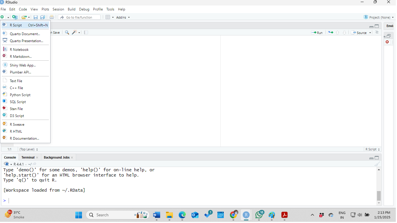
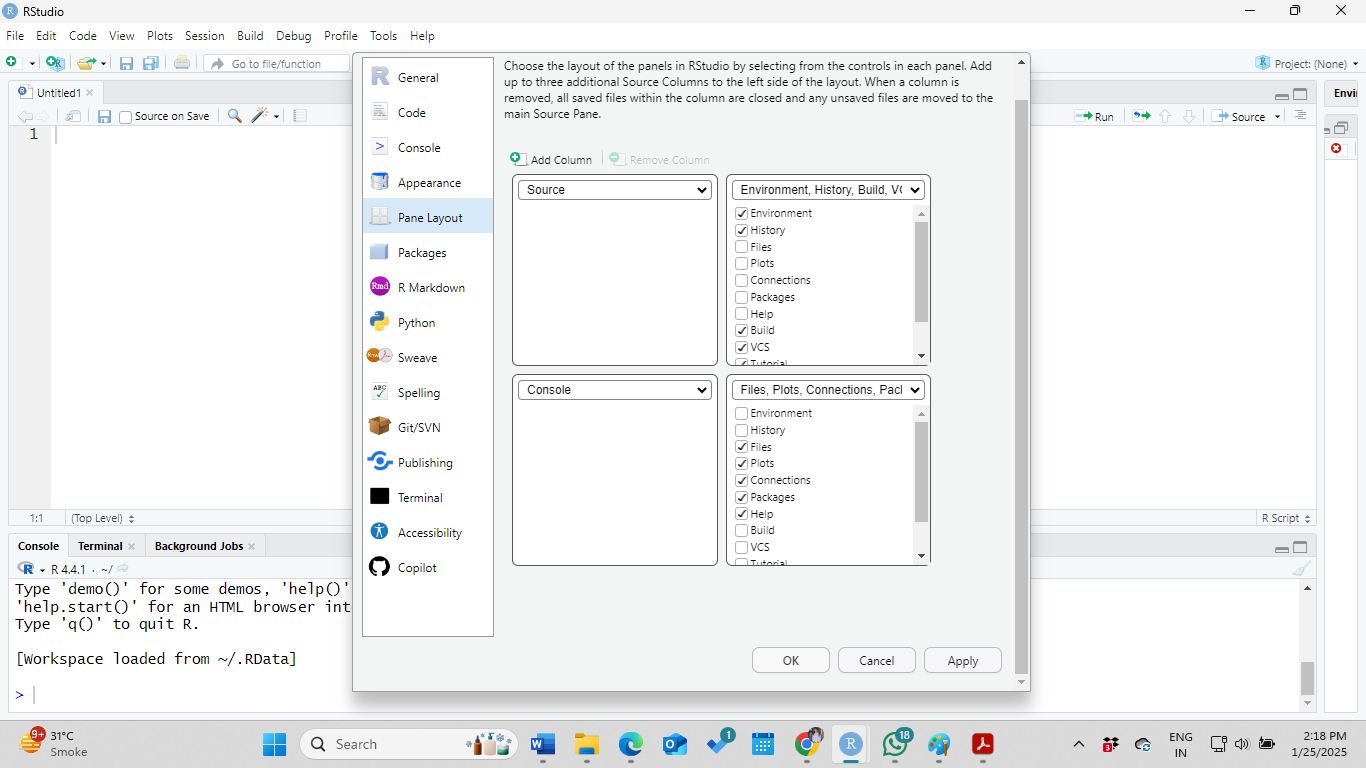
Typically, the look of RStudio contains four windows which are flexible that can be stretched or adjusted as the requirement of the user. However, the options in each pane can be customized by following the sequence: Tools -> Global Options -> Pane Layout
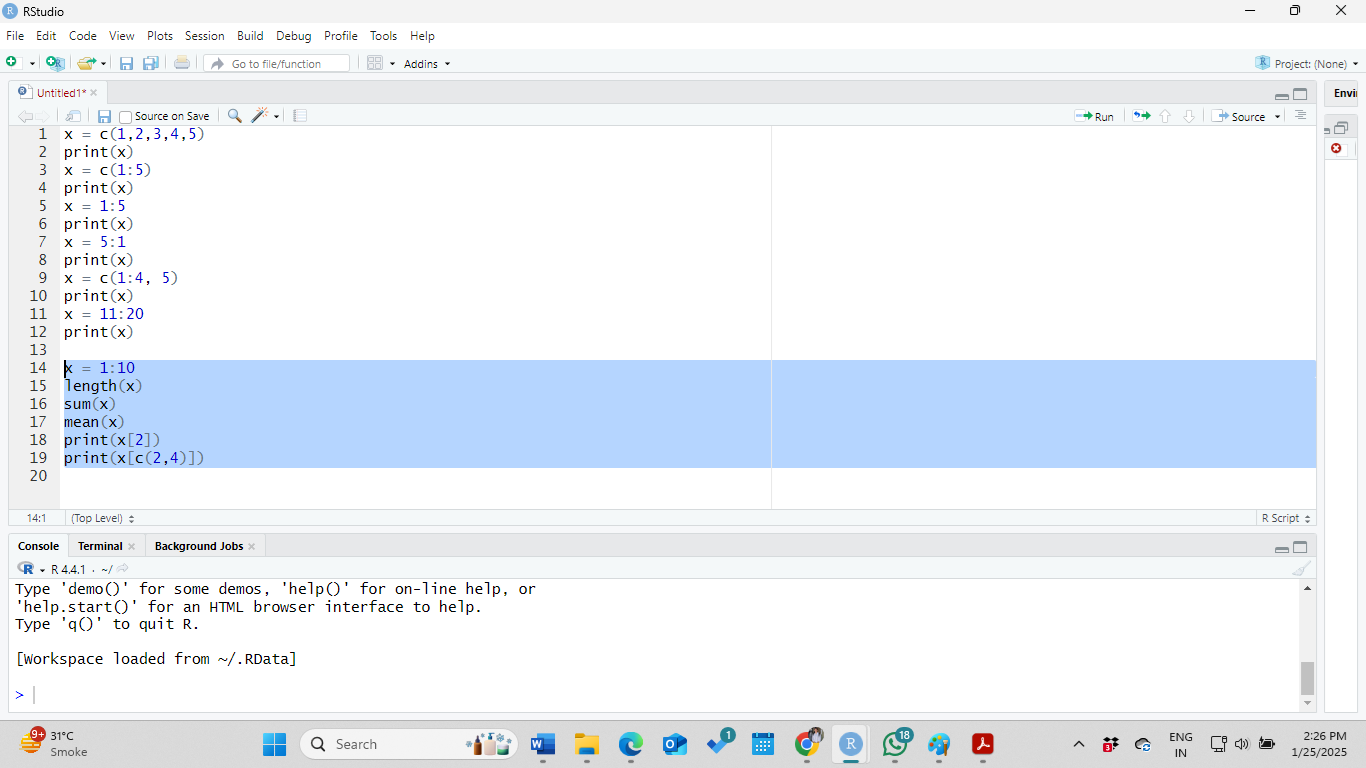
2.1.2 Concatenation Operator \(\texttt{c}\)
Execute the following codes and check the output in the console. The object \(\texttt{x}\) basically stores the numbers \(\{1,2,3,4,5\}\). There are multiple ways to store these numbers in \(\texttt{x}\).
2.1.3 Some basic inbuilt functions in R
The following functions will be helpful in basic operations on vectors or arrays in R. Below the above piece of codes, you can run the following codes as a continuation of the previous steps.
2.2 R as a calculator
In the following code snippet, we shall see that R can be used as basic calculators including basic mathematical functions
x = 3
print(x)

y = 5
print(y)

z = x + y
print(z)

u = x - y
print(u)

v = x/y
print(v)

w = x*y
print(w)
In the following some examples are provided involving common functions:
x = 2
log(x)
log(x, base = 2)
log10(x)
exp(x)
sin(x)
cos(x)
tan(x)
2.3 Array of numbers in R
x = 1:10
length(x)
sum(x)
mean(x)
print(x[2])
print(x[c(2,4)])
rev(x)                # reverse the numbers
cumsum(x)             # cumulative sum
prod(x)               # product of the numbers
cumprod(x)            # cumulative product of numbers

x = c(1,2,3,4,5)
print(x)
class(x)              # what type it is
length(x)             # length of the array
sum(x)                # sum of the numbers
x^2                   # square of all numbers
sqrt(x)               # square root of all the numbers
mean(x)               # average of these number
cumsum(x)             # cumulative sum
In the following, we see some mathematical operations of arrays.
x = 1:5
print(x)
y = 5:1
print(y)
z = x + y            # element wise addition
print(z)
u = x - y            # element wise subtraction
print(u)
v = x*y              # element wise multiplication
print(v)
w = x/y              # element wise division
print(w)
Although R provides direct addition of two sets of numbers if they are of same length or length of one array is a multiple of another array. We can explicitly write the codes how to perform element wise addition as given below:
x = 1:5                           # the first array
y = 5:1                           # the second array
length(x)
length(y)
length(x) == length(y)            # checking equality of length
z = numeric(length = length(x))   # initialization of array
print(z)
for (i in 1:length(x)) {          # for loop starts here
  z[i] = x[i] + y[i]
}
print(z)
There are multiple ways to create arrays in R with specific requirements based on the problem in hand. In the following, we show some examples.
x = 1:100
print(x)
x = seq(1, 100, by = 1)             # understand on your own
print(x)
y = seq(1, 100, by = 3)             # difference is same
print(y)
z = seq(0, 1, by = 0.1)             # creating a mesh for interval
print(z)
length(z)
w = seq(0, 1, length.out= 10)       # understand the difference with the previous
print(w)
length(w)

p = rep(1, 5)
print(p)
q = rep(1:5, each = 5)
print(q)
Missing values are very important to deal with in real life applications. In R, the missing values are indicated as NA. The function is.na() is used to check whether some entry in the data vector is missing or not. We can see some examples in the following:
x = c(1, 2, 3, NA, 5)
length(x)
is.na(x)
!is.na(x)
mean(x)                            # output NA
median(x)                            # output NA
sum(x)                             # output NA
prod(x)                            # output NA
It is important to note that if there is some missing information in the data, basic functions like mean(), sum() etc will not work. It will also return NA. Within the function include the option na.rm = TRUE, which indicates that there are missing values in the data. Therefore, the functions will compute the summary ignoring the missing values.
mean(x, na.rm = TRUE)
median(x, na.rm = TRUE)
sum(x, na.rm = TRUE)
prod(x, na.rm = TRUE)
var(x, na.rm = TRUE)            # variance of the data
sd(x, na.rm = TRUE)           # standard deviation of the data
2.4 Matrices in R
The \(\texttt{matrix()}\) function is used to create a matrix object with specific number of rows and columns.
m = 4                     # number of rows
n = 3                     # number of columns
A = matrix(data = NA, nrow = m, ncol = n)      # blank matrix
print(A)                                       # Contains NA
[,1] [,2] [,3]
[1,] NA NA NA
[2,] NA NA NA
[3,] NA NA NA
[4,] NA NA NAA[1,1] = 1 # Filling each position
A[1,2] = 2
A[1,3] = 3
A[2,1] = 4
A[2,2] = 5
A[2,3] = 6
A[3,1] = 7
A[3,2] = 8
A[3,3] = 9
A[4,1] = 10
A[4,2] = 11
A[4,3] = 12
print(A) [,1] [,2] [,3]
[1,] 1 2 3
[2,] 4 5 6
[3,] 7 8 9
[4,] 10 11 12Run the following codes and understand the functioning of each of the functions.
nrow(A)                        # number of rows
ncol(A)                        # number of columns
rowSums(A)                     # sum of each row
colSums(A)                     # sum of each column
rowMeans(A)                    # average of each row
colMeans(A)                    # average of each column
rownames(A) = c("R1", "R2", "R3", "R4")
print(A)
colnames(A) = c("C1", "C2", "C3")
print(A)
Suppose that we want to add the row sums and column sums in the same matrix and create a new one.
B = cbind(A, rowSums(A))                     # column bind
print(B)
C1 C2 C3
R1 1 2 3 6
R2 4 5 6 15
R3 7 8 9 24
R4 10 11 12 33colnames(B)[1] "C1" "C2" "C3" "" colnames(B)[4] = "RowSum" # add last column name
colnames(B) # check column names again[1] "C1" "C2" "C3" "RowSum"C = rbind(B, colSums(B)) # adding column sums
print(C) C1 C2 C3 RowSum
R1 1 2 3 6
R2 4 5 6 15
R3 7 8 9 24
R4 10 11 12 33
22 26 30 78rownames(C) [1] "R1" "R2" "R3" "R4" "" rownames(C)[5] = "ColSum" # add last row name
print(C) C1 C2 C3 RowSum
R1 1 2 3 6
R2 4 5 6 15
R3 7 8 9 24
R4 10 11 12 33
ColSum 22 26 30 782.4.1 Addition of two matrices
P = matrix(data = 1:9, nrow = 3, ncol = 3)
print(P)
[,1] [,2] [,3]
[1,] 1 4 7
[2,] 2 5 8
[3,] 3 6 9dim(P) # dimension of a matrix[1] 3 3Q = matrix(data = 11:19, nrow = 3, ncol = 3)
print(Q) [,1] [,2] [,3]
[1,] 11 14 17
[2,] 12 15 18
[3,] 13 16 19dim(Q)[1] 3 3dim(P) == dim(Q) # checking dimension[1] TRUE TRUER = matrix(data = NA, nrow = nrow(P),
ncol = ncol(P))
print(R) # blank matrix [,1] [,2] [,3]
[1,] NA NA NA
[2,] NA NA NA
[3,] NA NA NAfor (i in 1:nrow(P)) {
for (j in 1:ncol(P)) {
R[i,j] = P[i,j] + Q[i,j] # element wise addition
}
}
cat("The addition of the given matrices P and Q are\n", R)The addition of the given matrices P and Q are
12 14 16 18 20 22 24 26 28
Classroom Assignment: Matrix multiplication
Suppose that \(A\) is \(m\times n\) matrix and \(B\) is an \(n\times k\) matrices of real numbers. Write a programme to compute the product of these two matrices \(AB\) (matrix multiplication).
Using R write down the following to matrices \[E = \begin{bmatrix} 5.1 & 3.2 & 6.0 & 7.1 \\ 4.8 & 2.9 & 5.5 & 6.8 \\ 5.4 & 3.5 & 6.2 & 7.3 \\ \end{bmatrix}~~~~\mbox{and}~~~~W = \begin{bmatrix} 0.4 \\ 0.3 \\ 0.2 \\ 0.1 \\ \end{bmatrix}\]
Multiply these two matrix \(EW\) and report its dimension.
From each column of \(E\) subtract the column means and call it \(center_E\).
Consider the following piece of codes:
z = sample(1:1000, replace = TRUE)
print(z)
Check the \(\texttt{help(sample)}\) to gain knowledge about the
samplefunction.Pick out the values in
zwhich are greater than 600.What are the index positions in
zof the values which are greater than 600?Create a vector \[\left(|z_1-\bar{z}|^{1/2},|z_2-\bar{z}|^{1/2},\ldots,|z_n-\bar{z}|^{1/2}\right),\], where \(\bar{z}\) denotes the mean of the vector \(\mathrm{z}=(z_1,z_2,...,z_n)\)
How many numbers in
zare divisible by 2? (Note that the modulo operator is denoted %%.)Sort the numbers in the vector
zin the order of increasing values.Compute the following series
- \(\sum_{i=1}^5 \sum_{j=1}^15 \frac{i^3}{5+j}\)
- \(\sum_{i=1}^5 \sum_{j=1}^15 \frac{i^3}{5+ij}\)
- \(\sum_{i=1}^5 \sum_{j=1}^i \frac{i^3}{5+ij}\)
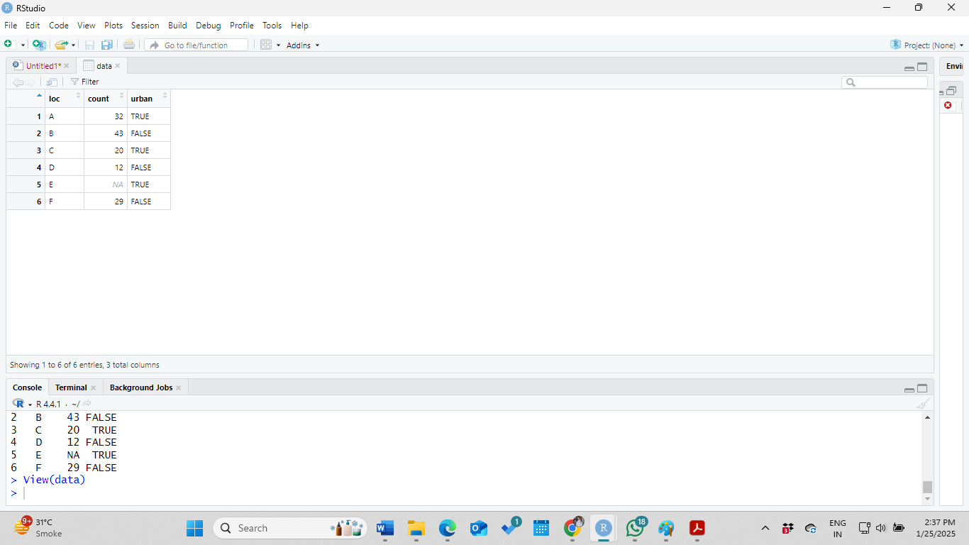
In ecological problems, we do always deal with numeric values, there are observations which are stored in strings as well. For example, we often collect data from different locations, and these identified by letters A, B, C, D. From these locations, the numbers of observations are 32, 43, 20 and 12, respectively. Therefore, to store this data, we need to have two vectors, one for locations and another for the counts. In addition, the location A and C are categorized as Urban and location B and D are categorized as Others. Therefore, we may require logical vector as well to store this information.
loc = c("A", "B", "C", "D")      # note inverted comma for characters
count = c(32, 43, 20, 12)          # numeric vector
urban = c(TRUE, FALSE, TRUE, FALSE)
print(loc)
print(count)
class(loc)                             # character vector
class(count)                           # numeric vector
class(urban)                           # logical vector
The function class() is a useful function to understand the type of the data and large scale data analysis problems often compatibility of different data types need to be checked. These three vectors are of same length equal to 5. However, they are now different objects, and we usually want to have an Excel view of these objects in a single dataset with multiple columns. In R, data.frame() function is used to create datasets.
data = data.frame(loc, count, urban)        # create dataset
print(data)
dim(data)                                             # dimension of data
nrow(data)                                          # number of rows
names(data)                                       # column names
ncol(data)                                          # number of columns
Suppose that we have information from another two locations E and F. E and F are categorized as urban and non-urban areas, respectively. From F the count is 29, however, from E, the count is not available. The new information can be added to the existing data in the following ways:
loc = c("E", "F")                               # new location
count = c(NA, 29)                               # counts
urban = c(TRUE, FALSE)                      # whether urban
new = data.frame(loc, count, urban)     # new data information
data = rbind(data, new)                     # adding to existing data
print(data)                                     # print in the console
You may would like to have an Excel kind of view.
There are important functions which directly helps to understand the structure of the data.
summary(data)
complete.cases(data)         # rows without missing information
!complete.cases(data)        # rows with missing information
data[,3]                     # third column of the data
data[1,2]
data[3,]                     # third row of the data
If you wish, you can also change the names of the rows and columns. The functions rownames() and colnames() are used to execute this task. Execute the following pieces of codes to understand their functionalities.
colnames(data) = c("Location", "Count", "Urban")
print(data)
rownames(data) = c("R1", "R2", "R3", "R4", "R5", "R6")
print(data)
A little understanding of the matrices is helpful in statistical modelling of the real data sets irrespective of the academic background. In the following codes, we see some operations on matrices and also learn how to create a matrix in R. Matrices are two dimensional arrangements of numbers and the dimension of a matrix A is 2×3, which means that the number of rows is 2 and the number of columns is 3. There is a total of six number are stored in the matrix. Let us create this matrix using the following codes:
A = matrix(data = 1:6, nrow = 2, ncol = 3)
print(A)
A[1,]                                      # First row of A
A[,3]                                      # Third column of A
A[1,3]                                 # number in the (1,3) position
dim(A)                             # dimension of A
nrow(A)                                # number of rows
ncol(A)                                # number of columns
rowSums(A)                             # sum of numbers in rows
colSums(A)                             # sum of numbers in columns
rowMeans(A)                          # average of numbers in rows
colMeans(A)                          # average of numbers in columns
sum(A)                                 # addition of all numbers in A
When the rows and columns are exchanged, we say the transpose operation on the matrix. Therefore, transpose of the matrix A, will contain the same numbers, but number of rows will be 3 and the number of columns will be 2.
t(A)
dim(t(A))
If two matrices A and B are of the same dimension, then they can be added or subtracted from each other. This operation is elementwise which means the (1,2) position number in A will be added (subtracted) with the (1,2) position number in B. If C = A+B, then C[1,2] = A[1,2]+B[1,2]. Similar will be followed for all other entries. The following example will demonstrate this fact:
A = matrix(data = 1:6, nrow = 2, ncol = 3)
B = matrix(data = 6:1, nrow = 2, ncol = 3)
C = A + B                                        # matrix addition
print(C)
D = A – B                                        # matrix subtraction
print(D)
E = A*B                                        # element wise multiplication
print(E)
F = A/B
print(F)                             # element wise division
If we have two matrices \(A\) and \(B\) as follows: \[ A = \begin{bmatrix} a_{11} & a_{12} \\ a_{21} & a_{22} \end{bmatrix},~ \text{and}~ B = \begin{bmatrix} b_{11} & b_{12} \\ b_{21} & b_{22} \end{bmatrix}. \]
Then, \[ A + B = \begin{bmatrix} a_{11} + b_{11} & a_{12} + b_{12} \\ a_{21} + b_{21} & a_{22} + b_{22} \end{bmatrix}. \]
\[ A \times B = \begin{bmatrix} a_{11} \times b_{11} & a_{12} \times b_{12} \\ a_{21} \times b_{21} & a_{22} \times b_{22} \end{bmatrix}. \]
Matrix multiplication, however, is different. Two matrices \(A\) and \(B\) of dimensions \(m \times n\) and \(p \times q\) can be multiplied if the number of columns in \(A\) is equal to the number of rows in \(B\), that is, \(n = p\). The resulting matrix will be of order \(m \times q\). In R, the symbol %*% is used to perform matrix multiplication.
For example: \[ A \%*\% B = \begin{bmatrix} a_{11} \times b_{11} + a_{12} \times b_{21} & a_{11} \times b_{12} + a_{12} \times b_{22} \\ a_{21} \times b_{11} + a_{22} \times b_{21} & a_{21} \times b_{12} + a_{22} \times b_{22} \end{bmatrix}.\]
A = matrix(data = 1:6, nrow = 3, ncol = 2)
print(A)
B = matrix(data = 1:6, nrow = 2, ncol = 3)
print(B)
ncol(A) == nrow(B)                     # condition of multiplication
C = A%*%B                                    # matrix multiplication
print(C)
dim(C)                                     # 3 by 3 matrix
A matrix is called a square matrix if the number of rows is equal to the number of columns of the matrix. The entries in the positions (1,1),(2,2), etc. are called diagonal entries. A matrix will diagonal entries 1 and off-diagonal entries as zero is called the identity matrix. In the following, A is a square matrix of order 3. Using the diag() function, we can obtain the diagonal entries.
A = matrix(data = 1:9, nrow = 3, ncol= 3)
diag(A)                                 # diagonal elements
If \(A\) and \(B\) are two square matrices of order \(n\), we say that \(B\) is the inverse of \(A\) (denoted by \(A^{-1}\)) if \(A\%*\%B=I=B\%*\%A\). The inverse matrix B can be obtained by the solve() function in R.
A = matrix(data = c(1,3,1,2,1,2,4,3,1), nrow = 3, ncol = 3)
print(A)
solve(A)                                   # inverse of A
eigen(A)                                   # eigenvalues of A
solve(A)%*%A                             # identity matrix
det(A)                                   # determinant of A
rowMeans(A)                            # average of each row
colMeans(A)                            # average of each column
colSums(A)                             # sum of each column
rowSums(A)                               # sum of each row
In above, we have seen data.frame and matrix objects in R. We observed that the matrix can not hold data of two different types. In another words, if we have two columns, one represents the abundance of some species (numeric) and the other represents the location of the site (in character). We cannot store this two information in a single matrix. Even if we store them, both the columns will be converted to character types. A small demonstration is shown below for understanding. The variable Density is a numeric variable, however, when it is stored in a matrix with another column Sites, the Density column is converted to character. In the print(M), observe that all the numbers are within inverted comma.
Density = c(100, 138, 80, 20, 41)     # numeric type
Sites = c("A", "B", "C", "D", "E")  # character type
M = cbind(Density, Sites)                 # Column binding
class(M)                                        # Matrix
class(M[,"Sites"])                        # character type
class(M[,"Density"])                # character type
class(Density)                              # numeric type
print(M)                                        # all within inverted comma
Apart from the data.frame and matrix, the knowledge of the list data structure also comes very handy in data analysis applications of R programming. You can think of list as a sequence of big containers. In each container, you can store different types of objects. For example, if you have a list of length 3, then in the first container, you can keep a matrix and in the second container, you can keep a data.frame and in the third container, you can keep a vector also.
List = list(length = 3)              # Empty list of length 3
D = data.frame(A = rep(c(1,2), 4), B = rnorm(n=8))
M = matrix(data = rnorm(n = 9), nrow = 3, ncol = 3)
x = 1:10
List[[1]] = D                              # First container
List[[2]] = M                              # Second container
List[[3]] = x                              # Third container
print(List)                              # print the list
2.4.2 Writing functions
It is important to have a basic idea of writing functions in R. Functions are often helpful to automate some data analysis process and help in reducing time for doing repetitive tasks. For example, I am interested in computing the average of the first and the last number of a set of values. The following code will do this task.
x = 1:10                                      # data values
(x[1] + x[10])/2                            # average of the first and last
Suppose the above process we want to do it for 5 sets of values and each of different lengths. Every time, we need to write this. However, if we write a function, the process can be done in much nicer way.
a = rep(1, 5)                               # repeat 1 five times
b = c(5:10)                               # numbers 5 to 10
c = rev(10:1)                               # 1,2,3,…,10
d = 1:20                                      # 1,2,3,…,20
f = function(x){                            # function in R
  (x[1] + x[length(x)])/2
}
f(a)                                            # Check the return value
f(b)
f(c)
f(d)
We can also do customization of the function. Suppose instead of numeric value someone enters a character in the entry, then the summation will not be computed and result in error. Inside the function body, we can add more comments.
e = c("A", "B", "C")
f(e)                                            # error and read the error
You can modify the function as follows. As you can see that you can add multiple conditions and modify the function as per your requirements.
f = function(x){                            # modified function
  if(!is.numeric(x) == TRUE)
    return("Can not compute: the input is not numeric.")
  else
    return((x[1]+x[length(x)])/2)
}
f(e)                                            # customized output
You can also write down mathematical functions. The common algebraic and trigonometric functions are available in R. Some common functions are sin(), cos(), log(), etc. In the following, we show an example. The curve() function is very important to understand when dealing with mathematical functions.
par(mfrow = c(1,2))
f = function(x){
  x^2*sin(10*x)                     # body of the function
}
curve(f(x), -1,1, col = "red", lwd = 3, cex.lab = 1.3,
      main = expression(x^3*sin(10*x)))

g = function(x){
  x^3
}
h = function(x){
  sin(10*x)
}
curve(g(x), col = "red", lwd = 3, -1, 1, cex.lab = 1.3,
      ylim = c(-1.2, 1.6), lty = 2)
curve(h(x), add = TRUE, col = "blue", lwd = 3, lty = 3)
legend("topleft", legend = c(expression(x^3), expression(sin(10*x))), bty = "n",
       lwd = c(3,3), col = c("red", "blue"), lty = c(2,3),
       cex = 0.8)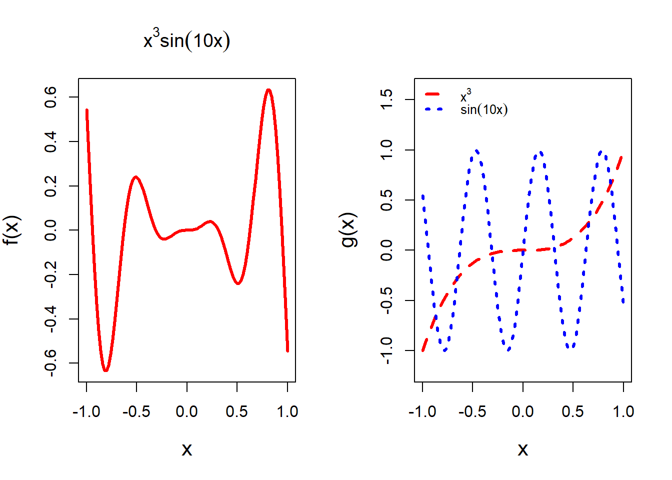
The curve function contains several important arguments, main, cex.main, add, lty, lwd, col, etc. You are encouraged to play with these options and see the changes in the plots. This hands-on experience will increase the comfort level in handling R programming tasks. You can add legends as well using the legend() function. The option bty = "n" specifies that we do not want to have a bounding box about the legend. The expression() function is useful for mathematical annotations in the plot window.
2.4.3 Some important functions in R
In the following, we list some common R functions which operates on the list of values in R. We give a small example, however, the same can be applied to large data sets as well.
x = c(rep(1,3), rev(1:5))
print(x)
which.max(x)
which.min(x)
which(x == 1)
which(x != 1)
sum(x == 1)
x[x == 1]
x[x!=1]
x[x > 1]
Run the above codes and interpret them on your own.
2.4.4 Symbolic computation
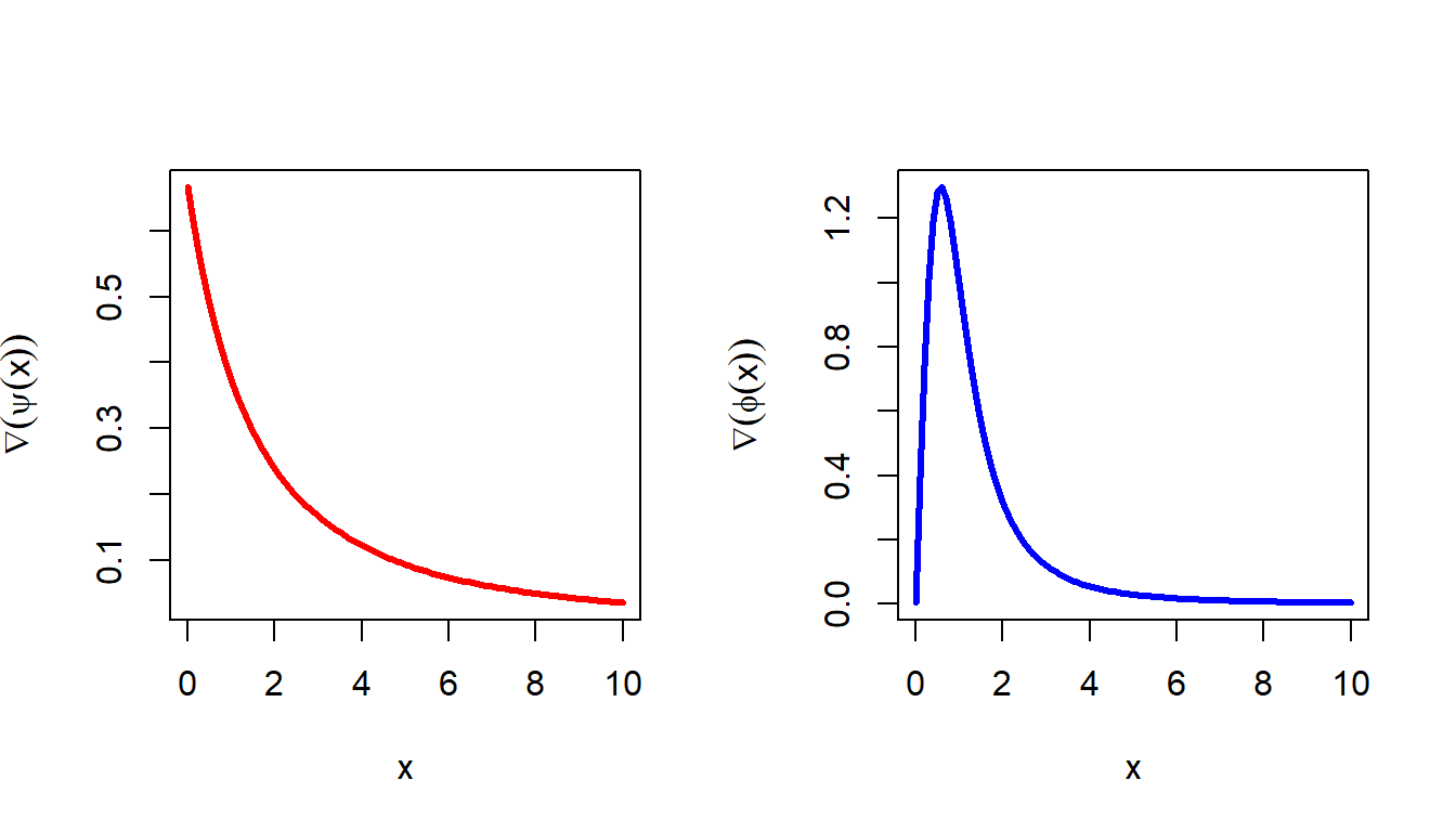
R also provides some options for performing symbolic computation. The operator D is used for this computation. In the following, we perform the symbolic derivative of the function \(\psi(x) = \frac{2x}{3+x}\) to compute \(\psi'(x)\) using R. Another example is also given with \(\psi(x) = \frac{2x^2}{1+x^2}\). We need to store the function within the expresion command.
par(mfrow = c(1,2))
expr = expression(2*x/(3+x))
cat("The derivative of the function is given by \n")
The derivative of the function is given by D(expr, 'x')2/(3 + x) - 2 * x/(3 + x)^2diff_psi = function(x){
(2/(3 + x) - 2 * x/(3 + x)^2)*(x>0)
}
expr = expression( ((2*x^2)/(1+x^2)))
cat("The derivative of the function is given by \n" )The derivative of the function is given by D(expr, 'x') 2 * (2 * x)/(1 + x^2) - (2 * x^2) * (2 * x)/(1 + x^2)^2diff_phi = function(x){
(2 * (2 * x)/(1 + x^2) - (2 * x^2) * (2 * x)/(1 + x^2)^2)*(x>0)
}
curve(diff_psi(x), col = "red", lwd = 3,
0.001, 10,
ylab = expression(nabla(psi(x))))
curve(diff_phi(x), col = "blue", lwd = 3,
0.001, 10, ylab = expression(nabla(phi(x))))