par(mfrow = c(1,2))
x = rnorm(n = 1000, mean = 0, sd = 1)
hist(x, probability = TRUE, breaks = 30)
y = x^2
hist(y, probability = TRUE, breaks = 30)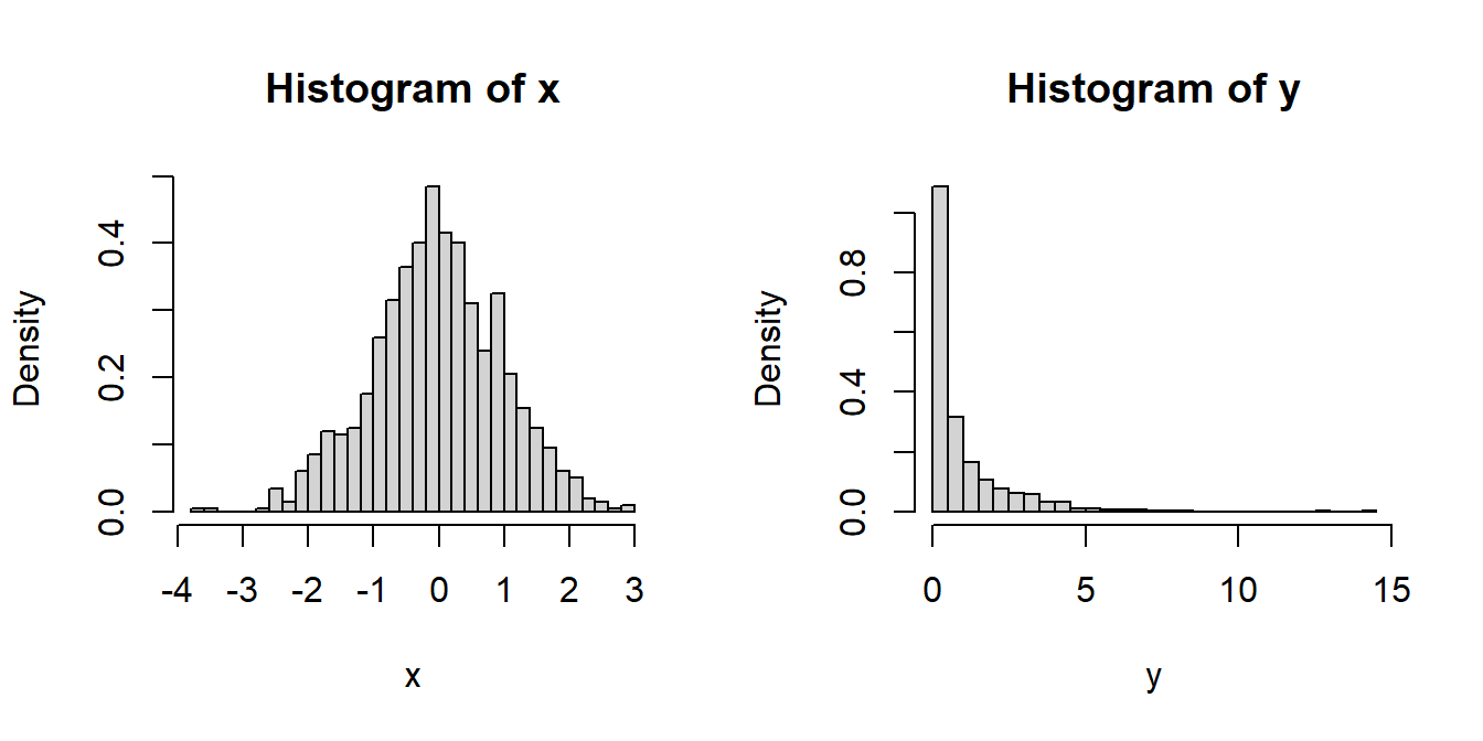
In the Chapter Introduction to Probability Distribution, we have learnt about the basic ideas about the probability mass function and the probability density function. Suppose that we have a random variable \(X\) with the probability density function \(f_X(x)\) and we are interested in obtaining the PDF of \(Y=g(X)\), which is a transformation of the random variable \(X\). To start this concept, we start with an illustrative example.
Suppose that \(X\sim \mathcal{N}(0,1)\) and we aim to find the probability distribution of \(Y = X^2\). We can think of the \(Y\) as the squared distance of the random variable \(X\) from \(0\). We define the support of a random variable \(X\) as set of all points on the real line for which the PDF \(f_X(x)\) is positive and denoted by the symbol \(\mathcal{X}\). Therefore, \[\mathcal{X} = \{x\in \mathbb{R}\colon f_X(x)>0\}.\]
\(Y\) is a transformation of \(X\) and we define the sample space of \(Y\) as \[\mathcal{Y}=\{y\in \mathbb{R}\colon f_Y(y)>0\}.\]
In this context we have \(g(x)=x^2\), \(\mathcal{X} = (-\infty,\infty)\) and \(\mathcal{Y}=(0,\infty)\). Before going into the mathematical computations, let us do some simulation and try to see whether the distributions show some commonly known patterns. From an algorithmic point of view, we do the following steps:
par(mfrow = c(1,2))
x = rnorm(n = 1000, mean = 0, sd = 1)
hist(x, probability = TRUE, breaks = 30)
y = x^2
hist(y, probability = TRUE, breaks = 30)It can be observed that the simulated realizations from the distribution of \(Y\) is highly positively skewed. Let us try to obtain the PDF of \(Y\) by explicit computation. We take the following strategy:
\[\begin{eqnarray} F_Y(y) &=& \mbox{P}(Y\le y) = \mbox{P}(X^2\le y)\\ &=&\mbox{P}\left(-\sqrt{y}\le X\le \sqrt{y}\right)\\ &=& 2\mbox{P}(0\le X\le \sqrt{y})~~(\mbox{even function})\\ &=& 2\times \int_0^{\sqrt{y}}\frac{1}{\sqrt{2\pi}}e^{-\frac{x^2}{2}}dx \end{eqnarray}\]
It is worthwhile to remember the Leibnitz rule for differentiation under the integral sign: \[\frac{d}{dy}\int_{a(y)}^{b(y)}\psi(x,y)dx = \psi\left(b(y),y\right)b'(y)-\psi\left(a(y),y\right)a'(y)+\int_{a(y)}^{b(y)} \frac{\partial}{\partial y} \psi(x,y)dx,\] provided the required mathematical requirements on the function \(\psi(x,y)\) is satisfied.
The PDF of \(Y\) is given by \[f_Y(y) = \frac{e^{-\frac{y}{2}}y^{\frac{1}{2}-1}}{\Gamma\left(\frac{1}{2}\right)2^{\frac{1}{2}}}, 0<y<\infty,\] and zero otherwise. The important observation is that the square of the standard normal distribution belongs to the \(\mathcal{G}(\alpha,\beta)\) family of distributions. Let us expand this problem in a two dimensional scenarios.
During the lecture, we post the following question: Suppose that we consider the two dimensional plane and call \((x_1,x_2)\) plane. We have \(X_1 \sim \mathcal{N}(0,1)\) and \(X_2 \sim \mathcal{N}(0,1)\) and we are interested to compute the probability that \(\mbox{P}\left(X_1^2 +X_2^2\le 1\right)\). Let us understand this probability statement in a simple language: Suppose we randomly choose a point on the \((x_1,x_2)\) plane, where each coordinate is chosen randomly and independently from the \(\mathcal{N}(0,1)\) distribution, what is the probability that the selected point will fall within the circle of unit radius. There are two strategies to compute this probability.
First idea is more intuitive rather than mathematically rigorous. We consider the following steps to be performed using R
par(mfrow = c(1,2))
m = 1000
x1 = rnorm(n = m, mean = 0, sd = 1)
x2 = rnorm(n = m, mean = 0, sd = 1)
plot(x1, x2, pch = 19, col = "grey",
     xlab = expression(x[1]), ylab = expression(x[2]))
abline(h = 0, col = "red", lwd = 2)
abline(v = 0, col = "red", lwd = 2)
y = x1^2 + x2^2
curve(sqrt(1-x^2), -1 ,1, col = "blue", lwd = 2, lty = 2,
      add = TRUE)
curve(-sqrt(1-x^2), -1 ,1, col = "blue", lwd = 2, lty = 2,
      add = TRUE)
cat("Approximate probability based on m = 1000 simulated data point is ", mean(y<=1))
Approximate probability based on m = 1000 simulated data point is 0.398hist(y, probability = TRUE, breaks = 30)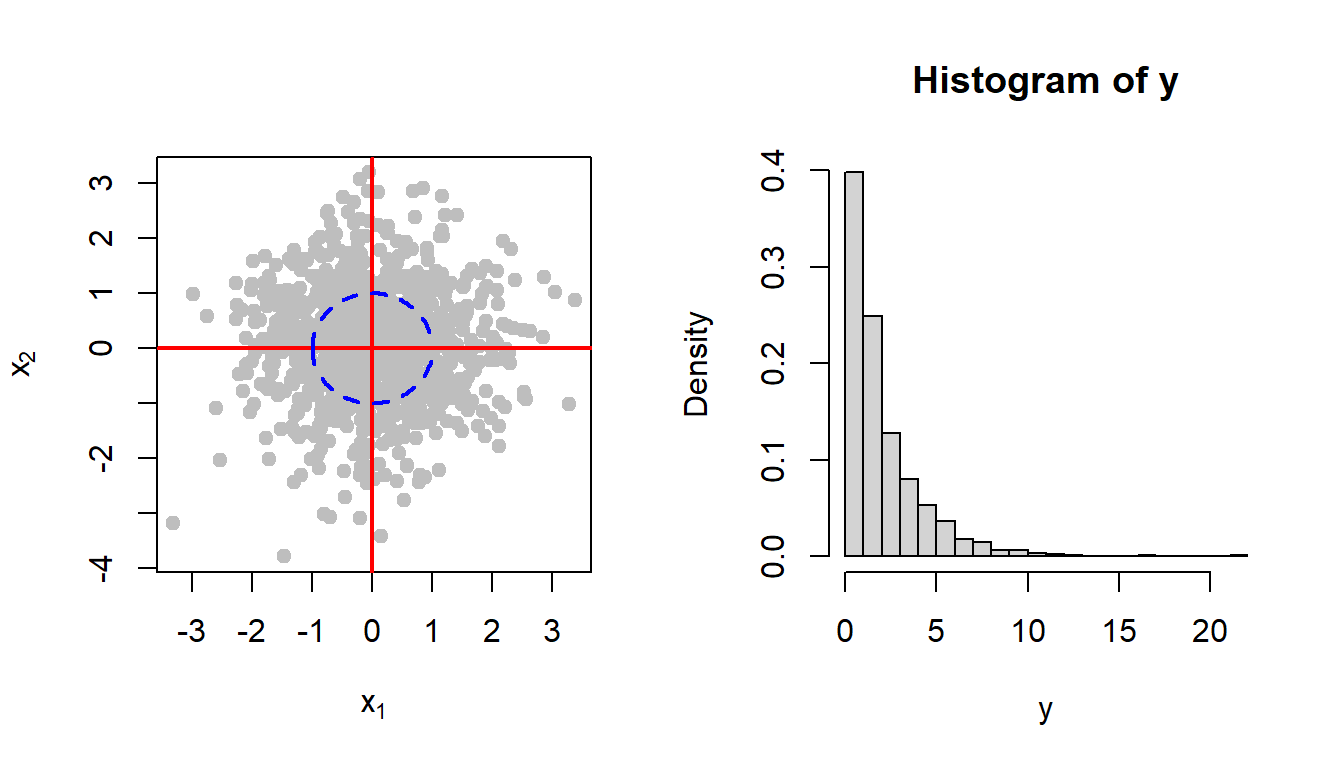
The above simulation scheme suggested a highly positively skewed distribution for the random variable \(Y\). Let us try to compute the exact PDF of \(Y\). We have already learnt how to compute \(f_Y(y)\) by computing the CDF from the definition. In this case, the following integration needs to be carried out: \[F_Y(y) = \mbox{P}\left(X_1^2 + X_2^2\le y\right)= \int\int_{\left\{(x_1,x_2)\colon x_1^2+x_2^2\le y\right\}}\frac{1}{2\pi}e^{-\frac{1}{2}\left(x_1^2+x_2^2\right)}dx_1dx_2.\] You are encouraged to perform this integration, however, we can try some alternative approach as well. For example, we now understood that both \(X_1^2\) and \(X_1^2\) follows \(\sim \mathcal{G}\left(\alpha = \frac{1}{2}, \beta = 2\right)\) and \(Y\) is nothing but sum of two independent \(\mathcal{G}(\cdot, \cdot)\) distributions. We recollect the moment generating function of the \(\mathcal{G}(\alpha, \beta)\), where \(\alpha\) and \(\beta\) are the shape and scale parameters, respectively. The MGF is given by \[M(t) = (1-\beta t)^{-\alpha}, t<\frac{1}{\beta}.\] In addition, the expected value and variance of this distribution is \(\alpha\beta\) and \(\alpha \beta^2\), respectively.
Suppose that \(W_1 \sim \mathcal{G}(\alpha_1, \beta)\) and \(W_2\sim \mathcal{G}(\alpha_2, \beta)\) and \(W_1\), \(W_2\) are independent random variables and let \(W = W_1 +W_2\). Then the MGF of \(W\) is can be computed as \[\begin{eqnarray} M_W(t) &=& \mbox{E}\left(e^{tW}\right) = \mbox{E}\left(e^{tW_1 + tW_2}\right)\\ &=& \mbox{E}\left(e^{tW_1}\right)\mbox{E}\left(e^{tW_2}\right) = M_{W_1}(t)M_{W_2}(t) ~~(\mbox{independence})\\ & =& (1-t\beta)^{-(\alpha_1 + \alpha_2)}, ~~t<\frac{1}{\beta}. \end{eqnarray}\] Therefore, \(W \sim \mathcal{G}(\alpha_1+\alpha_2,\beta)\); in particular the addition of these two independent random variables also belonging to the \(\mathcal{G}\) family of distributions. Using this result, we can see that \[Y = X_1^2 + X_2^2 \sim \mathcal{G}\left(\alpha = 1, \beta = 2\right).\] Let us check whether the theory is matching with the simulated histograms of the \(Y\) values in the previous figure.
par(mfrow = c(1,2))
m = 1000
x1 = rnorm(n = m, mean = 0, sd = 1)
x2 = rnorm(n = m, mean = 0, sd = 1)
plot(x1, x2, pch = 19, col = "grey",
     xlab = expression(x[1]), ylab = expression(x[2]))
abline(h = 0, col = "red", lwd = 2)
abline(v = 0, col = "red", lwd = 2)

y = x1^2 + x2^2
hist(y, probability = TRUE, breaks = 30)
curve(dgamma(x, shape = 1, scale = 2), add = TRUE,
      col = "red", lwd = 2)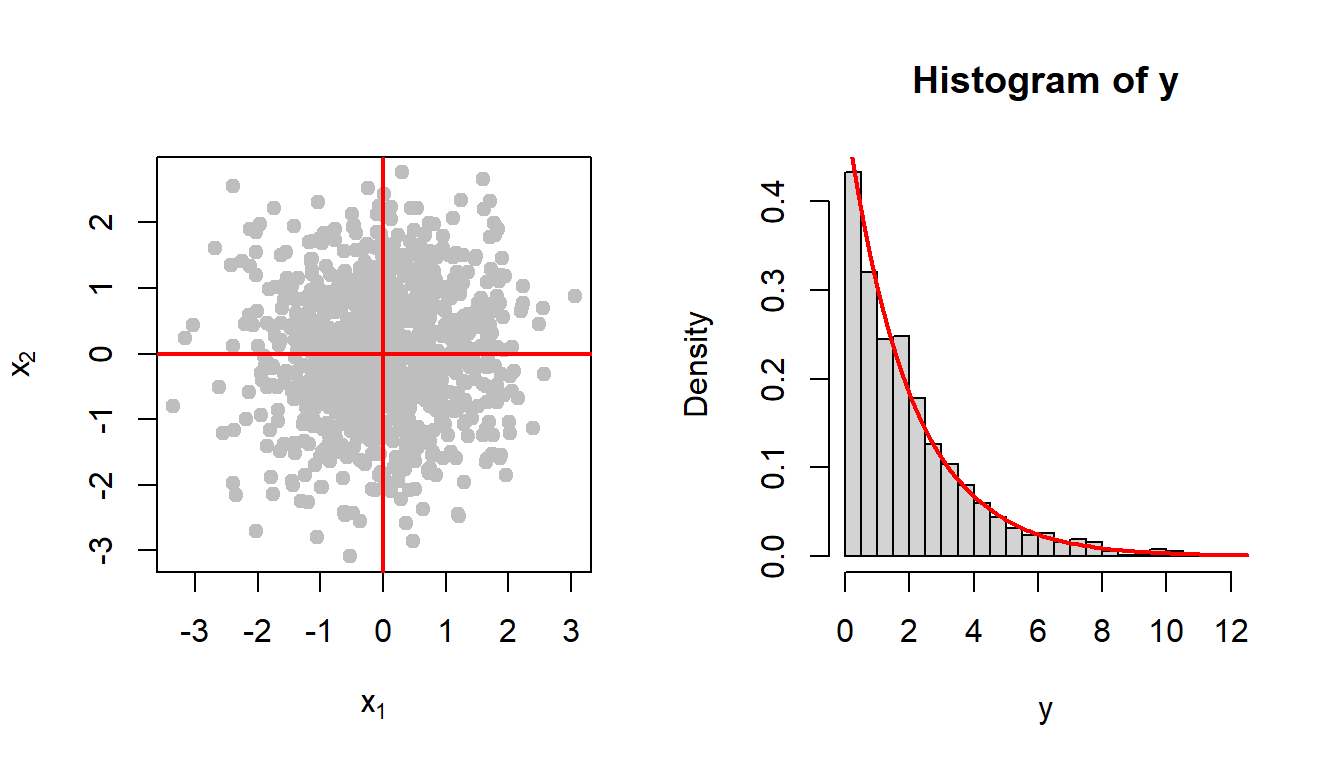
I believe, now are in a position to generalize this idea. We just extend the idea using an important result which states that if \(W_i \sim \mathcal{G}(\alpha_i,\beta)\) for \(1\le i\le n\) and they are independent, then \[\sum_{i=1}^nW_i \sim \mathcal{G}\left(\alpha_1+\cdots+\alpha_n, \beta\right).\]
Let us write them in a sequential manner:
Therefore, for \(n\in \mathbb{N}\), the PDF of \(Y_n\) is given by \[f_{Y_n}(y) = \frac{e^{-\frac{y}{2}}y^{\frac{n}{2}-1}}{2^{\frac{n}{2}}\Gamma\left(\frac{n}{2}\right)}, 0<y<\infty,\] and zero otherwise. This probability density function is celebrated as the chi-squared distribution with \(n\) degrees of freedom and usually denoted as \(Y_n \sim \chi^2_n\). From the properties of the \(\mathcal{G}(\cdot,\cdot)\) distribution, we can easily conclude that \[\mbox{E}(Y_n) = n,~~Var(Y_n) = \frac{n}{2}\times 2^2 = 2n.\] Let us visualize the distribution of the \(Y_n\) for different choices of \(n\) values based on \(m=1000\) replications.
par(mfrow = c(2,3))
n_vals = c(2,5, 10, 30, 40, 100)
for(n in n_vals){
  m = 1000
  sim_data = matrix(data = NA, nrow = m, ncol = n)
  for(j in 1:n){
    sim_data[,j] = rnorm(n = m, mean = 0, sd = 1)
  }
  # head(sim_data)
  y = numeric(length = m)
  for (i in 1:m) {
    y[i] = sum(sim_data[i,]^2)
  }
  hist(y, probability = TRUE, main = paste("n = ", n),
       breaks = 30, col = "lightgrey")
  curve(dgamma(x, shape = n/2, scale = 2),
        add = TRUE, col = "red", lwd = 2)

}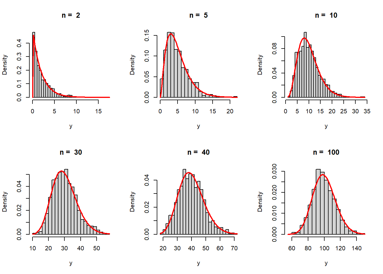
While these histograms are well approximated by the \(\chi^2_n\) distribution, one student noticed that as \(n\) increases, the histograms and the PDFs are behaving similar to bell curve, that is the normal distribution. Therefore, a natural question arises, is the \(\chi^2_n\) PDF looks like a bell curve for large \(n\)? In addition, what will be mean and variance of this bell curve if these distributions are well approximated by bell curve. For experiment purpose, let us draw the \(\chi^2_n\) PDF and the normal PDF with mean \(n\) and variance \(2n\), that is \(\mathcal{N}(n,2n)\) for different choices of \(n\). The functions dgamma(), dchisq(), dnorm() suggest the uniform use of the letter d in plotting the density function in R.
par(mfrow = c(2,3))
n_vals = c(2,8,10,30,50,100)
for(n in n_vals){
  curve(dchisq(x, df = n), col = "red", lwd = 2,
        xlim = c(n-4*sqrt(2*n),n+4*sqrt(2*n)), main = paste("n = ", n),
        ylab = expression(f(x)))
  curve(dnorm(x, mean = n, sd = sqrt(2*n)),
        add = TRUE, col = "blue", lwd = 2, lty = 2)
  legend("topright", legend = c(expression(chi[n]^2), "N(n,2n)"),
         col = c("red", "blue"), lwd = c(2,2), lty = c(1,2), bty = "n")
}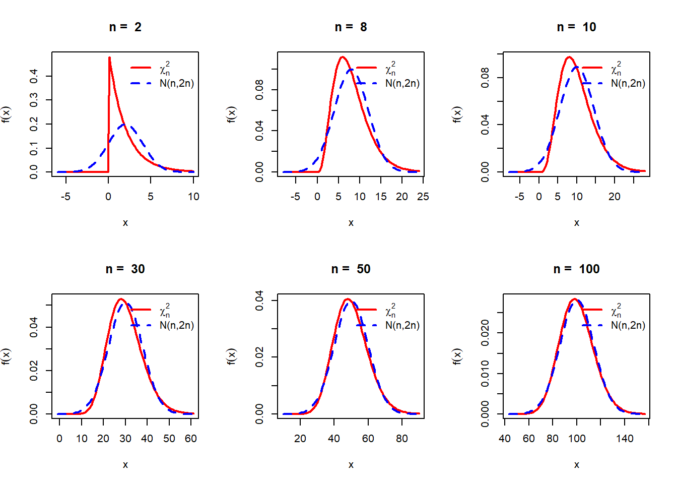
For a theoretical proof of the above observations, we can prove in the class that for large \(n\), the Moment Generating Function of \(\frac{X-n}{\sqrt{2n}}\) is approximately equal to \(e^{\frac{t^2}{2}}\) which is the MGF of the standard normal distribution. Since \(\frac{X-n}{\sqrt{2n}}\sim \mathcal{N}(0,1)\) for large \(n\), therefore, \(X \sim \mathcal{N}(n,2n)\) for large \(n\).
It is important to plot the curves of the PDFs for different choices of the parameters.
The probability integral transform is a fundamental theorem in statistical simulation. Suppose that we are interested in simulating random numbers from the distribution of \(X\), whose CDF is given by \(F_X(x)\), say. If we consider the transformation \(U = F_X(X)\), basically, the transformation function \(g(\cdot)\) is the CDF itself \(F_X(\cdot)\), then \(U\sim \mbox{Uniform}(0,1)\). This is quiet surprising as the result is true for any random variable. Therefore, if we simulate \(U\sim \mbox{Uniform}(0,1)\), then we can obtain a realization from the distribution of \(X\), by considering the following inverse transformation: \[X = F_X^{-1}(U).\] We must take caution in defining the inverse mapping \(F_X^{-1}\) of \(F_X\). For example, if \(X\) is a discrete random variable, then \(F_X(x)\) is a step function, therefore, the inverse can not be defined in usual sense. We will not discuss it further here and close this session with an illustrative example using the exponential(1) distribution. The CDF is given by \(F_X(x) = 1-e^{-x}, 0\le x<\infty\) and zero for \(x<0\). Therefore, for \(F_X^{-1}(U) = -\log(1-U), 0<U<1\). The following code is used to demonstrate the simulation of exponential(1) random variables starting with the \(\mbox{Uniform}(0,1)\) random numbers.
CDF_Exp = function(x){
  (1 - exp(-x))*(x>0)
}
# curve(CDF_Exp(x), -1, 6, col = "red", lwd = 2)

par(mfrow = c(2,3))
n = 1000
x = rexp(n = n, rate = 1)
hist(x, probability = TRUE)
plot(ecdf(x), ylab = expression(F[n](x)))
curve(CDF_Exp(x), -1, 6, col = "red", lwd = 2,
      add = TRUE)

U = CDF_Exp(x)
head(U)
[1] 0.2177833 0.3923647 0.8961038 0.2549403 0.8819981 0.3040599hist(U, probability = TRUE)
curve(dunif(x), add = TRUE, col = "red", lwd = 2)
inv_CDF_Exp = function(u){
-log(1-u)
}
U = runif(n = n)
hist(U, probability = TRUE)
x = inv_CDF_Exp(U)
plot(ecdf(x), col = "grey", ylab = expression(F[n](x)))
curve(CDF_Exp(x), -1, 6, col = "red", lwd = 2, add = TRUE)
hist(x, probability = TRUE)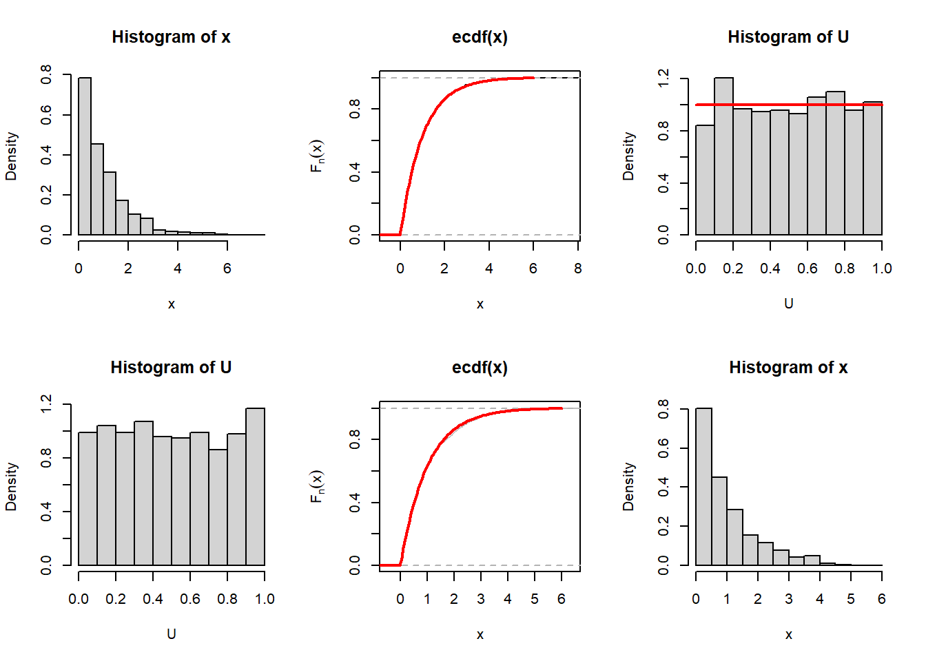
Suppose \(U_1\) and \(U_2\) are two independent uniformly distributed random variables from the interval \((0,t)\) for \(t>0\). We are interested to understand the sampling distribution of the \(\max\left(U_1,U_2\right)\) and \(\min\left(U_1,U_2\right)\). In the following code, we simulate the sampling distribution of these two functions. You are encouraged to simulate the sampling distributions for the maximum and minimum of \(n\) independent and identically distribution \(\mbox{Uniform}(0,t)\) random variables. These are also called the maximum and minimum order statistics and typically denoted as \(U_{(n)}\) and \(U_{(1)}\), respectively.
t = 3
U = runif(n=2, min = 0, max =t)
n = length(U)
U1 = min(U)
U2 = max(U)
print(U1)
[1] 1.210107print(U2)[1] 1.814647M = 10000
U1 = numeric(length = M)
U2 = numeric(length = M)
for (i in 1:M) {
U = runif(n=2, min = 0, max =t)
U1[i] = min(U)
U2[i] = max(U)
}
f_U2 = function(x){
n*(x/t)^(n-1)*(1/t)*(0<x)*(x<t)
}
f_U1 = function(x){
n*(1-x/t)^(n-1)*(1/t)*(0<x)*(x<t)
}
par(mfrow=c(1,3))
hist(U1, probability = TRUE, xlim = c(0,t),
breaks = 30, xlab = expression(U[1]),
main = expression(f[U[(1)]](u[1])))
curve(f_U1, add = TRUE, col = "red", lwd = 2)
hist(U2, probability = TRUE, xlim = c(0,t),
breaks = 30, xlab = expression(U[2]),
main = expression(f[U[(2)]](u[2])))
curve(f_U2, add = TRUE, col = "red", lwd = 2)
library(gplots)
hist2d(U1, U2, col = c("green", heat.colors(12)),
xlab = expression(U[(1)]), ylab = expression(U[(2)]))
----------------------------
2-D Histogram Object
----------------------------

Call: hist2d(x = U1, y = U2, col = c("green", heat.colors(12)), xlab = expression(U[(1)]),
    ylab = expression(U[(2)]))

Number of data points:  10000
Number of grid bins:  200 x 200
X range: ( 0.0002591943 , 2.935092 )
Y range: ( 0.04063615 , 2.999993 )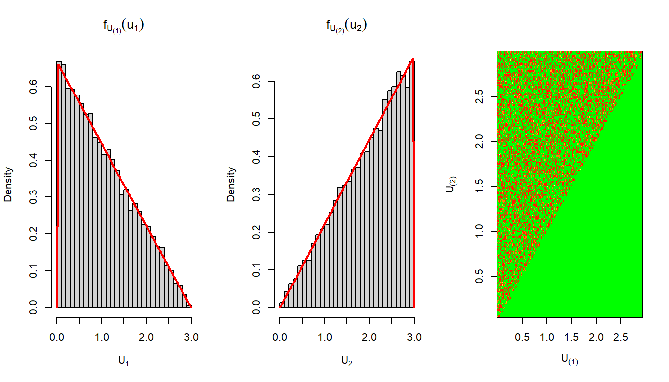
You are encouraged to execute the following code to understand that the how different is the two dimensional histogram of \(\left(U_{(1)}, U_{(2)}\right)\) than the histogram of random numbers simulated from the joint distribution of \(\left(U_1, U_2\right)\)
# IID Uniform(0,t)
U1 = runif(n = M, min = 0, max = t)
U2 = runif(n = M, min = 0, max = t)
hist2d(U1, U2, col = c("green", heat.colors(12)),
       xlab = "U1", ylab = "U2")