p = 0.3                                 # probability of head
n = 100                                 # number of throws
x = rbinom(n = n, size = 1, prob = p)   # coin tossing experiment
print(x)                                # 1 = head, 0 = tail
sum(x) # number of heads14 Interdisciplinary Teaching of Statistical Data Science
In many data science workshops, the instructor usually provides readymade code that participants simply run, often without fully understanding how it works. Also, when a workshop has too many speakers or unrelated sessions, participants can find it hard to follow the overall flow.
This chapter describes a different kind of approach, designed especially for ecologists, more generally to the interdisciplinary audience. The focus here is on learning through live discussions, practical examples, and writing code together. All the codes shown in this chapter were written live during the workshop, not prepared in advance and the participants wrote the same code alongside the instructor in real time. The goal was to help participants think critically and connect statistics to their own research. The case studies in this chapter reflect that interactive approach, showing how hands on learning can make statistical ideas clearer and more useful for ecologists. The case studies in this chapter reflect that interactive approach, showing how hands-on learning can make statistical ideas clearer and more useful, not just for ecologists, but for a broader interdisciplinary audience working with real world data.
14.1 Statistical Distributions
Probability distributions play a fundamental role in real-life data analysis problems. However, their importance is often underestimated in many applications, leading students to blindly accept the outcomes provided by software. Understanding probability distributions equips us with the ability to grasp the inherent uncertainty in natural processes. Data collected from the field are subject to various types of randomness, and probability theory provides a framework for these random phenomena. In this manual, we shall understand various probability distributions using R without getting into the mathematical intricacies of these distributions.
To understand the distribution theory using R, we need to learn about the four letters in R: r, d, p, q. We start our discussion with the coin tossing experiments. Suppose we want to simulate a coin tossing experiment using R instead of performing that experiment physically. Suppose the probability of success is \(p=0.3\). If we toss the coin 100 times say, we should expect an approximately 30 many heads (intuition!). In the following, we do this experiment once and observe that how many heads have been obtained. Certainly, the assumption that such experiments can be identically performed an infinitely many numbers of times remain intact. As an applied researcher, we should just keep these statements as universally true.
You are required to check whether the sum is actually 30 or not. If it appeared to be 30, do this experiment once again, you are likely to get another number, however, that is expected to be close to 30. As an ecologist, each run of the above code may be considered as follows: I visited a site consecutively 100 days and, on each day, we record 1 if we observe a phenomenon of our interest, otherwise record 0. Although, it is highly superficial to consider that conditions of all the 100 are identical, but somewhere, we need to start the discussion also to get into a more complicated statistical thinking.
In the above code the quantity x contains a possible realization of coin tossing experiment (called Bernoulli trial). Out of 100 positions, each position can be filled with 2 ways (either 0 or 1). Therefore, there are a total \(2^{100}\) possible realizations of the coin tossing experiment. Similarly, in observations on the phenomenon of your interest, out of \(2^{100}\) possibilities, we have obtained a particular sequence of 0’s and 1’s, which we call as the field observations. The \(\mbox{Bernoulli}(p)\) distribution essentially acts as a probability model for the natural process from which we have collected the observations. Our interest may be to get an accurate estimate of the unknown probability \(p\) (with certain confidence!).
Statisticians often say to ecologists that if you provide more data then he/she could give you better estimates. This is not a magic. This simple coin tossing experiment itself may reveal this justification adequately. Suppose that we toss the coin n times and record the number of successes, then obtain the proportion of success as an estimate of \(p\). We then increase the number n and see whether, the proportion of success becomes close to the true probability 0.3 using which the simulation experiment has been carried out. We need to have cautionary note here, in the field experiment we never (ever) know what the underlying truth, that is what is the exact value of probability of observing the phenomena. However, in a computer simulation, we know that the experiments have performed by setting \(p=0.3\). Therefore, we can verify whether the proportion of success gets closer to the true value as the sample size increases. The following example will demonstrate this fact:
p = 0.3                                           # true probability
n_vals = 1:1000                                   # sample size
p_hat = numeric(length = length(n_vals))          # sample proportion
for(n in n_vals){
  x = rbinom(n = n, size = 1, prob = p)           # simulate coin tossing
  p_hat[n] = sum(x)/n                             # proportion of success
}
plot(n_vals, p_hat, type = "l", xlab = "sample size (n)",
     ylab = expression(widehat(italic(p))), col = "grey",
     cex.lab = 1.3, lwd = 2)
abline(h = p, col = "blue", lwd = 2, lty = 2)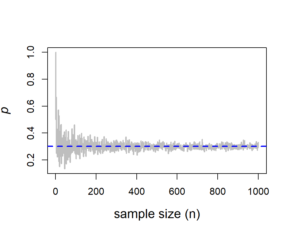
In the above code snippet, we observed the use for loop, numeric() function, mathematical annotation using expression(), use of colour in plots, abline() function for horizontal line plot, etc. We have used to letter r to simulate random numbers from the Bernoulli(p) experiment. Similarly, we can simulate random numbers from the desired probability distributions. Now we discuss the favorite bell-shaped curve: the normal distribution which appears everywhere! The normal distribution is characterized by the two quantities mean \(\mu\) and variance \(\sigma^2\). The quantity \(\mu\) can be any real number, where as the variance must be bigger than zero. First, we simulate n=100 random numbers from the normal distribution with parameters \(\mu=3\) and \(\sigma^2=1\). Note that the square-root of the variance is the standard deviation (denoted as sd).
par(mfrow = c(1,3))                            # side by side plot
mu = 3                                         # mean
sigma = 1                                      # sd
n = 100                                        # sample size
x = rnorm(n = n, mean = mu, sd =sigma)         # simulate numbers
hist(x, probability = TRUE, main = "", cex.lab = 1.4)
curve(dnorm(x, mean = mu, sd = sigma), lwd = 2,
      col = "red", add = TRUE)                 # add normal PDF
legend("topright", legend = "N(3,1)", lwd = 2,
       col = "red", bty = "n")                 # add legend

mu = 3                                         # mean
sigma = 2                                      # standard deviation
n = 100                                        # sample size
x = rnorm(n = n, mean = mu, sd = sigma)        # simulate observations
hist(x, probability = TRUE, main = "", cex.lab = 1.4)
curve(dnorm(x, mean = mu, sd = sigma), lwd = 2,
      col = "red", add = TRUE)
legend("topright", legend = "N(3,2)", lwd = 2,
       col = "red", bty = "n")

mu = 0
sigma = 1
n = 100
x = rnorm(n = n, mean = mu, sd = sigma)
hist(x, probability = TRUE, main = "", cex.lab = 1.4)
curve(dnorm(x, mean = mu, sd = sigma), lwd = 2,
      col = "red", add = TRUE)
legend("topright", legend = "N(0,1)", lwd = 2,
col = "red", bty = "n") # add legend 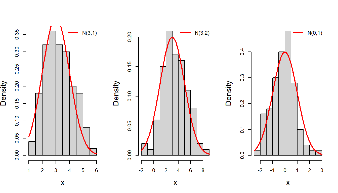
You are encouraged to execute the following codes, to understand the role of letter r in simulation of random numbers in R.
n = 100                                           # sample size
x = rexp(n = n, rate = 1)                         # simulation of exponential rv
hist(x, probability = TRUE)                       # histogram
curve(dexp(x, rate = 1), add = TRUE)              # adding the exact PDF
help("rexp")                                      # get help in R

n = 100
x  = runif(n = n, min = 0, max = 2)               # simulation of uniform(0,2)
hist(x, probability = TRUE)
curve(dunif(x, min =0, max = 2), add = TRUE)
help("dunif")

n = 100
x = rgamma(n = n, shape = 3, rate = 2)            # simulation of Gamma(3,2)
hist(x, probability = TRUE)
curve(dgamma(x, shape = 3, rate = 2), add = TRUE)
help("rgamma")
14.1.1 Poisson distribution
The Poisson distribution commonly appears in the ecological problems that deals with the count data. For example, ecologists studying the ant colonies often assume that the number of eggs laid by an individual ant follows a Poisson distribution with rate parameter \(\lambda>0\) (which is the parameter of interest). For the Poisson distribution, the mean and variance of the distribution are same (\(\lambda\)). Applications of Poisson distribution also appears in studying the distribution of rare plants in large forests (Krebs, Charles J. 1999. “Ecological Methodology.” 2nd ed. Benjamin-Cummings). The following code can be used to simulate random numbers from the Poisson distribution with fixed rate parameter \(\lambda\).
par(mfrow = c(1,1))
n = 100                                                 # sample size
lambda = 4                                              # rate parameter
x = rpois(n = n, lambda = lambda)                       # simulate Poisson RV
print(x)
Using the function dpois(), we can draw the Poisson probability mass function. The following code will do this task.
par(mfrow = c(1,2))                                     # side by side plot
x = 0:15
lambda = 2                                              # rate parameter
prob = dpois(x, lambda = lambda)                        # Poisson probability
plot(x, prob, type = "h", col = "grey", lwd = 2,
     cex.lab = 1.3, ylab = "P(X=x)",
     main = expression(paste(lambda, " = 2")))
points(x, prob, pch = 19, cex = 1.5, col = "blue")      # add points to existing plot

lambda = 5                                              # rate parameter
prob = dpois(x, lambda = lambda)                        # Poisson probability
plot(x, prob, type = "h", col = "grey", lwd = 2,
     cex.lab = 1.3, ylab = "P(X=x)",
     main = expression(paste(lambda, " = 5")))
points(x, prob, pch = 19, cex = 1.5, col = "blue")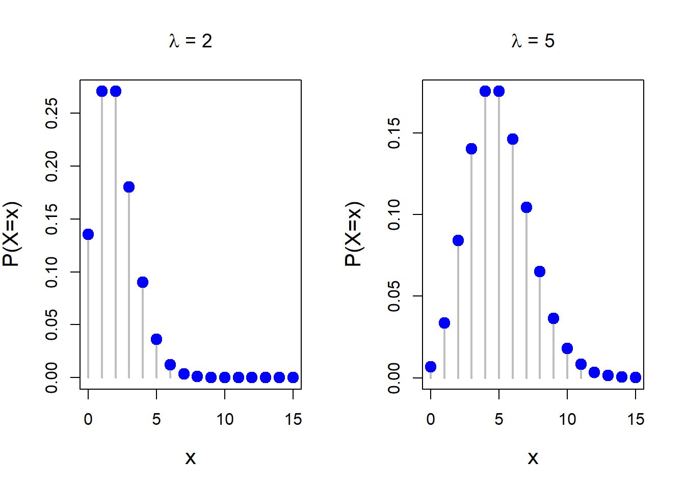
dpois() have been used to compute the exact probability values for the Poisson distribution at each value from the set {0,1,2,…,15}.
14.2 Modelling and Simulation
Mathematical models are commonly used to model the growth process in natural sciences and these models often include a stochastic component to incorporate the uncertainty inherent in the natural processes. Regression models play important role in ecological data analysis. To demonstrate the next statistical model fitting exercises, we consider the following data set which is available in R. The following
data("trees")
head(trees)                                # first six observations
summary(trees)                             # summary of the data set
dim(trees)                                 # data dimension
complete.cases(trees)                      # checking for missing rows
tail(trees)                                # last six observations
class(trees)
names(trees)                               # names of the columns
head(trees, n = 10)                        # first ten observations
tail(trees)                                # last six observations
str(trees)                                 # structure of the data frame
This data set provides measurements of the diameter, height and volume of timber in 31 felled black cherry trees. Note that the diameter (in inches) is erroneously labelled Girth in the data. The data set is available in datasets package in R. Before starting any analysis, it is very important to get an understanding of the data set with different visualization techniques.
par(mfrow=c(1,2))
data("trees")
summary(trees)                                 # data summary
Girth Height Volume
Min. : 8.30 Min. :63 Min. :10.20
1st Qu.:11.05 1st Qu.:72 1st Qu.:19.40
Median :12.90 Median :76 Median :24.20
Mean :13.25 Mean :76 Mean :30.17
3rd Qu.:15.25 3rd Qu.:80 3rd Qu.:37.30
Max. :20.60 Max. :87 Max. :77.00 boxplot(trees, col = 2:4, main = "Box plot")
library(vioplot) # violin plot
vioplot(trees, col = 2:4, main = "Violin plot")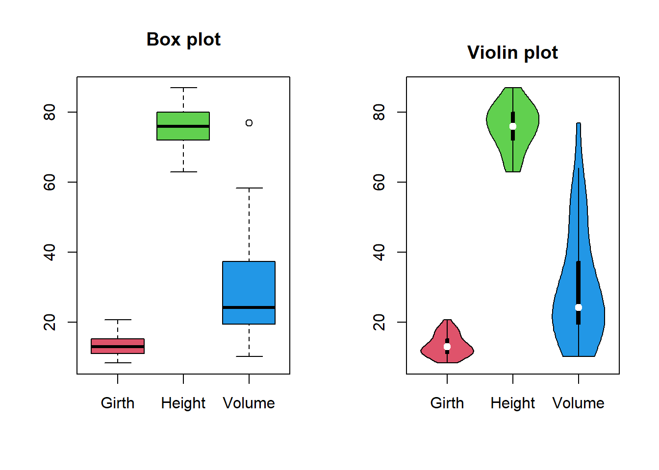
Often histograms are also utilized for visualization of the data distribution of the observations. The following code can be used to draw the histograms. It is to be noted that the $ symbol is used to access the columns from the data.frame in R.
par(mfrow = c(1,3))
hist(trees$Girth, probability = TRUE, main = "",
     xlab = "Girth", cex.lab = 1.3, col = 2)                   # histogram of Girth
hist(trees$Height, probability = TRUE, main = "",
     xlab = "Height", cex.lab = 1.3, col = 3)                  # histogram of height
hist(trees$Volume, probability = TRUE, main = "",
     xlab = "Volume", cex.lab = 1.3, col = 4)                  # histogram of volume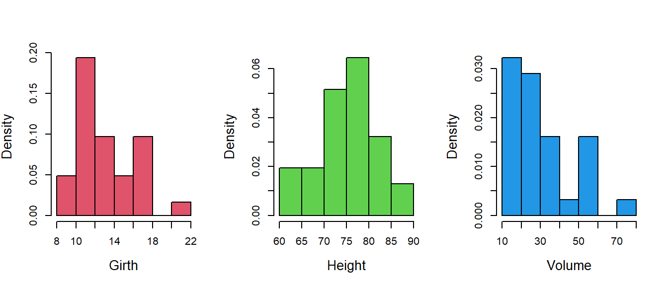
Exploring the relationship between different columns in the data set is often considered as the first step of modelling exercises. As a research statement, we may consider that whether the Girth and Height of a tree are a good predictor of the Volume. The pairs() function is a magical function in R that gives a great visual representation to explore the pairwise relationship of variables in the data.
pairs(trees, col = "red", pch = 19)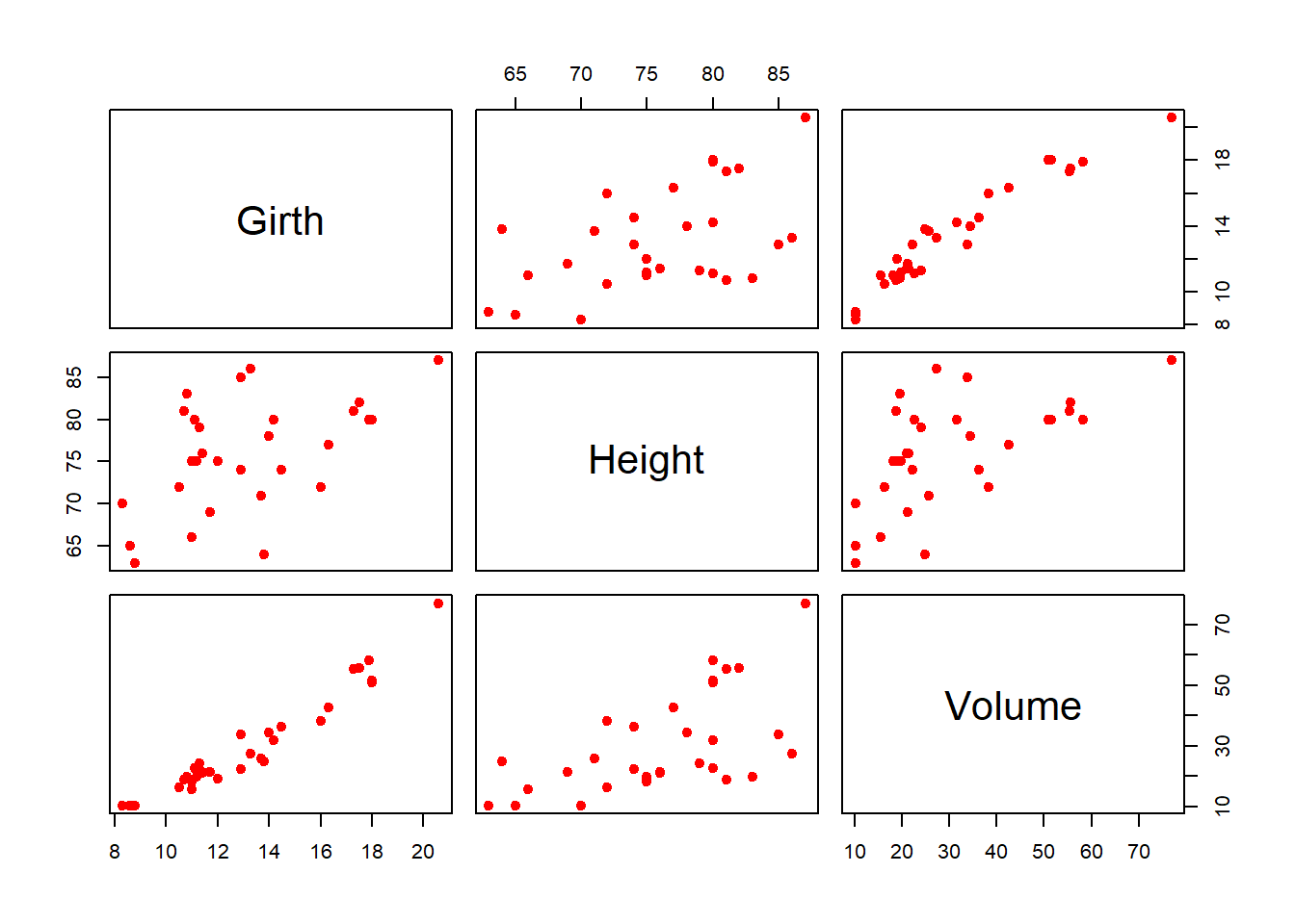
There are interesting packages in R that allows to explore the correlations between variables with great visualizations. The package corrplot allows great flexibility in presentation of correlation between variables. The following codes will help you to understand different varieties of representation of the correlation matrix.
par(mfrow = c(2,3))
library(corrplot)
corrplot(cor(trees))
cor(trees)
Girth Height Volume
Girth 1.0000000 0.5192801 0.9671194
Height 0.5192801 1.0000000 0.5982497
Volume 0.9671194 0.5982497 1.0000000#help("corrplot")
corrplot(cor(trees), method = "number")
corrplot(cor(trees), method = "number", type = "upper")
corrplot(cor(trees), method = "ellipse", type = "upper")
corrplot(cor(trees), method = "pie")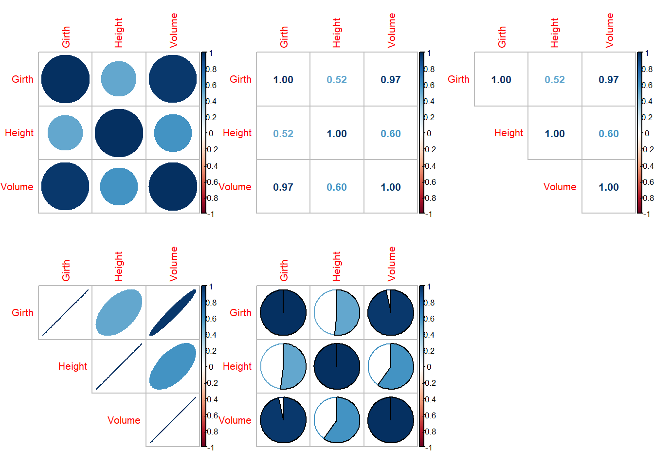
14.2.1 apply family of functions
The apply family of functions is an important way of computing various statistical characteristics of the data. Suppose that we are interested in computing the median of each column of the dataset. Individually, we can take each column of the data and compute it. However, the following code will help it to do it quickly.
apply(X = trees, MARGIN = 2, FUN = mean)             # column means
apply(X = trees, MARGIN = 2, FUN = median)           # column medians
apply(X = trees, MARGIN = 2, FUN = sd)               # column sd
In the apply function, MARGIN = 2 corresponds to the columns, whereas MARGIN = 1 corresponding to the rows.
In the first step of the analysis, suppose we aim to predict the Volume of the timber using the tree diameter. Therefore, we consider following statistical model
\[\text{Volume} = \beta_0 + \beta_1\times\text{Girth} + \epsilon. \tag{14.1}\]
In the above expression, Volume is the response variable and Girth is the predictor variable. \(\beta_0\) and \(\beta_1\) are the intercept and the slope parameters of the population regression line, respectively. The \(\epsilon\) represents the random component that cannot be explained through the linear relationship between the response and predictor. We also assume that \(\epsilon\sim \mathcal{N}(0, \sigma^2)\). In the above equation, Girth is fixed and \(\epsilon\) is random, which makes the Volume as a random quantity and follows normal distribution with mean \(\beta_0 + \beta_1\times\text{Girth}\) and variance \(\sigma^2\).
It is very important to note that assumption of such relationships at the population level mostly driven by the visualization and existing knowledge pool about the underlying process. In this case, from the scatterplot, we have hypothesized that a linear relationship between the Volume and the Girth may be a reasonable assumption to consider. In principle, the true nature of the relationship is always unknown. With our scientific instruments, we can probably identify a most likely relationship from a set of reasonable hypotheses. However, in this case, our visualization is quite clear, and we go ahead with the assumption of linear relationships.
Our goal is to estimate the parameters \(\beta_0\), \(\beta_1\) and \(\sigma^2\). There are 31 observations, and we write down the data model as
\[\text{Volume}_i = \beta_0 + \beta_1\times\text{Girth}_i + \epsilon_i, i\in\{1,2,\ldots,n\}.\]
We seek to obtain the estimate of \(\beta_0\) and \(\beta_1\) that minimizes the error sum of squares:
\[\sum_{i=1}^{31}(\text{Volume}_i- \beta_0 - \beta_1\times\text{Girth}_i)^2.\]
Using R, we can estimate the parameters of the interest. The following code will do this task for us. In this case, we have only one predictor and one response, therefore, it is called as a simple linear regression. The function lm() understand the formula Volume ~ Girth as an input and identifies which one is response and which one is predictors.
fit = lm(formula = Volume ~ Girth, data = trees)
coefficients(fit)                                     # estimated coefficients
(Intercept) Girth
-36.943459 5.065856 summary(fit) # summary of the fitting
Call:
lm(formula = Volume ~ Girth, data = trees)

Residuals:
   Min     1Q Median     3Q    Max
-8.065 -3.107  0.152  3.495  9.587

Coefficients:
            Estimate Std. Error t value Pr(>|t|)
(Intercept) -36.9435     3.3651  -10.98 7.62e-12 ***
Girth         5.0659     0.2474   20.48  < 2e-16 ***
---
Signif. codes:  0 '***' 0.001 '**' 0.01 '*' 0.05 '.' 0.1 ' ' 1

Residual standard error: 4.252 on 29 degrees of freedom
Multiple R-squared:  0.9353,    Adjusted R-squared:  0.9331
F-statistic: 419.4 on 1 and 29 DF,  p-value: < 2.2e-16
The most important part in the output to understand the interpretation of the p-value which is represented as Pr(>|t|). The fitting exercise also perform the testing of two hypotheses \[\mbox{H}_0: \beta_0 = 0 ~\text{versus}~ \mbox{H}_1: \beta_0\neq 0\] \[H_0: \beta_1 = 0 ~\text{versus}~ H_1: \beta_1\neq 0\]
If reject the null hypothesis \(\mbox{H}_0: \beta_1 = 0\) (at certain level of significance, say \(5\%\)), that means the tree diameter (Girth) has a good contribution in predicting the volume of timber.***indicates that the tree diameter is highly significant in determining the volume of timber. The same interpretation goes to the intercept as well. A multiple R-squared value of 0.9353 indicates that the approximately \(94\%\) of the variation in the Volume can be explained by the tree diameter through a linear function. In this case, this is quite satisfactory.
par(mfrow = c(1,2))
plot(Volume ~ Girth, data = trees, col = "red", pch = 19)
abline(fit, col = "blue", lwd = 2)

resid = residuals(fit)                                    # residuals of fit
hist(resid, probability = TRUE, xlab = "residuals",
     main = "")
shapiro.test(resid)                                         # test for normality
    Shapiro-Wilk normality test

data:  resid
W = 0.97889, p-value = 0.7811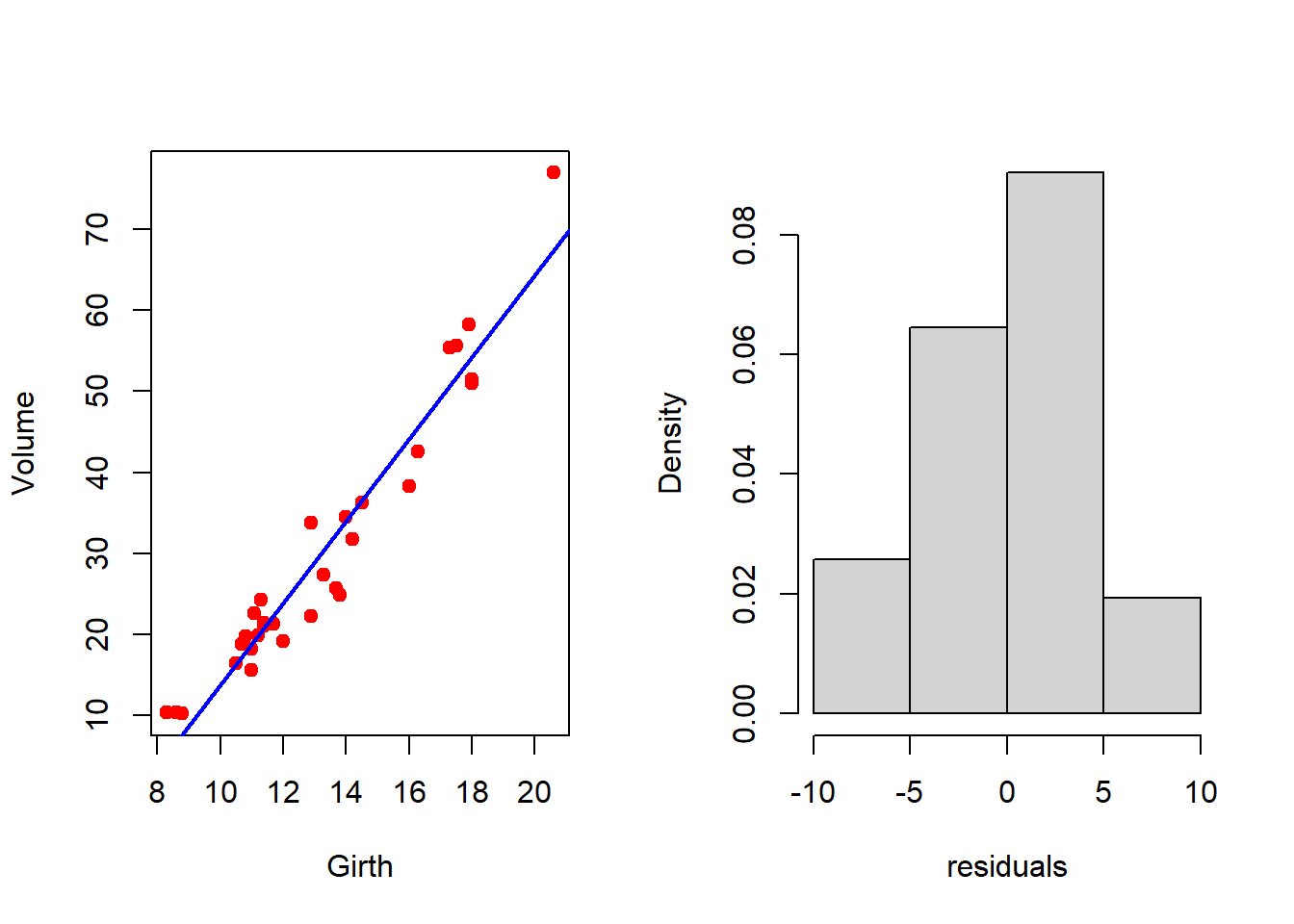
It is important to check whether the error is normally distributed. We have used the shapiro.test() to check for the normality. A large p-value indicates the acceptance of the null hypothesis that is the errors are normally distributed. After the fitting exercises, the regression diagnostics must be performed to check the validity of the assumptions that we have made at the starting of the discussion. Using the following piece of codes, we can get a visualization of the regression diagnostic tools.
par(mfrow = c(2,2))
plot(fit, pch = 19, col = "blue", lwd = 2)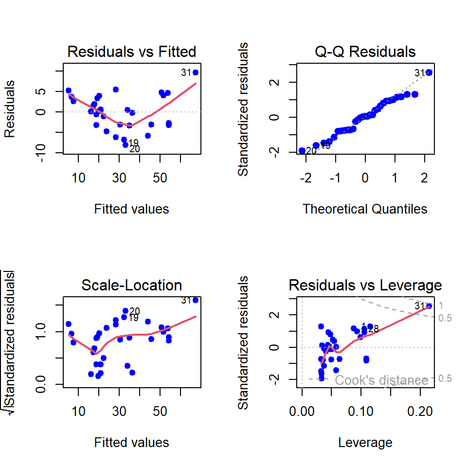
Although we have obtained the coefficient of determination (\(R^2\)) is approximately \(94\%\), the residual versus fitted plot gives a slight indication of nonlinearity. Suppose we plan to make this model quadratic in the following way:
\[\text{Volume} = \beta_0 + \beta_1\times\text{Girth} + \beta_2\times\text{Girth}^2 + \epsilon. \tag{14.2}\]
Note that in this case, the model complexity increases (with additional parameter \(\beta_2\) to be estimated). The other assumptions remain the same. The same function lm() in R can be utilized to estimate the parameters. We utilize the wrapper I(.) to include the polynomial expression in R.
par(mfrow = c(1,2))
fit2 = lm(formula = Volume ~ Girth + I(Girth^2),
          data = trees)                             # quadratic fit
summary(fit2)                                             # fit summary
Call:
lm(formula = Volume ~ Girth + I(Girth^2), data = trees)

Residuals:
    Min      1Q  Median      3Q     Max
-5.4889 -2.4293 -0.3718  2.0764  7.6447

Coefficients:
            Estimate Std. Error t value Pr(>|t|)
(Intercept) 10.78627   11.22282   0.961 0.344728
Girth       -2.09214    1.64734  -1.270 0.214534
I(Girth^2)   0.25454    0.05817   4.376 0.000152 ***
---
Signif. codes:  0 '***' 0.001 '**' 0.01 '*' 0.05 '.' 0.1 ' ' 1

Residual standard error: 3.335 on 28 degrees of freedom
Multiple R-squared:  0.9616,    Adjusted R-squared:  0.9588
F-statistic: 350.5 on 2 and 28 DF,  p-value: < 2.2e-16
By considering quadratic regression model, the coefficient of determination has increased to \(96\%\) from \(94\%\). However, the p-values suggest that the intercept and first order component do not have significant contribution in explaining the variation in Volume of timber through a quadratic regression model. It essentially says that the model is as good as having the expression as Volume= \(\beta_2\times\text{Girth}+\epsilon\).
par(mfrow = c(1,2) )
plot(Volume ~ Girth, data = trees,
     col = "red", pch = 19)                          # original data
lines(trees$Girth, fitted.values(fit2),
      col = "blue", lwd = 2)                         # fitted curve
resid2 = residuals(fit2)                               # residuals
hist(resid2, probability = TRUE, xlab = "residuals",
     main = "")                                          # residual distribution
shapiro.test(resid2)                                     # test for normality
    Shapiro-Wilk normality test

data:  resid2
W = 0.97393, p-value = 0.6327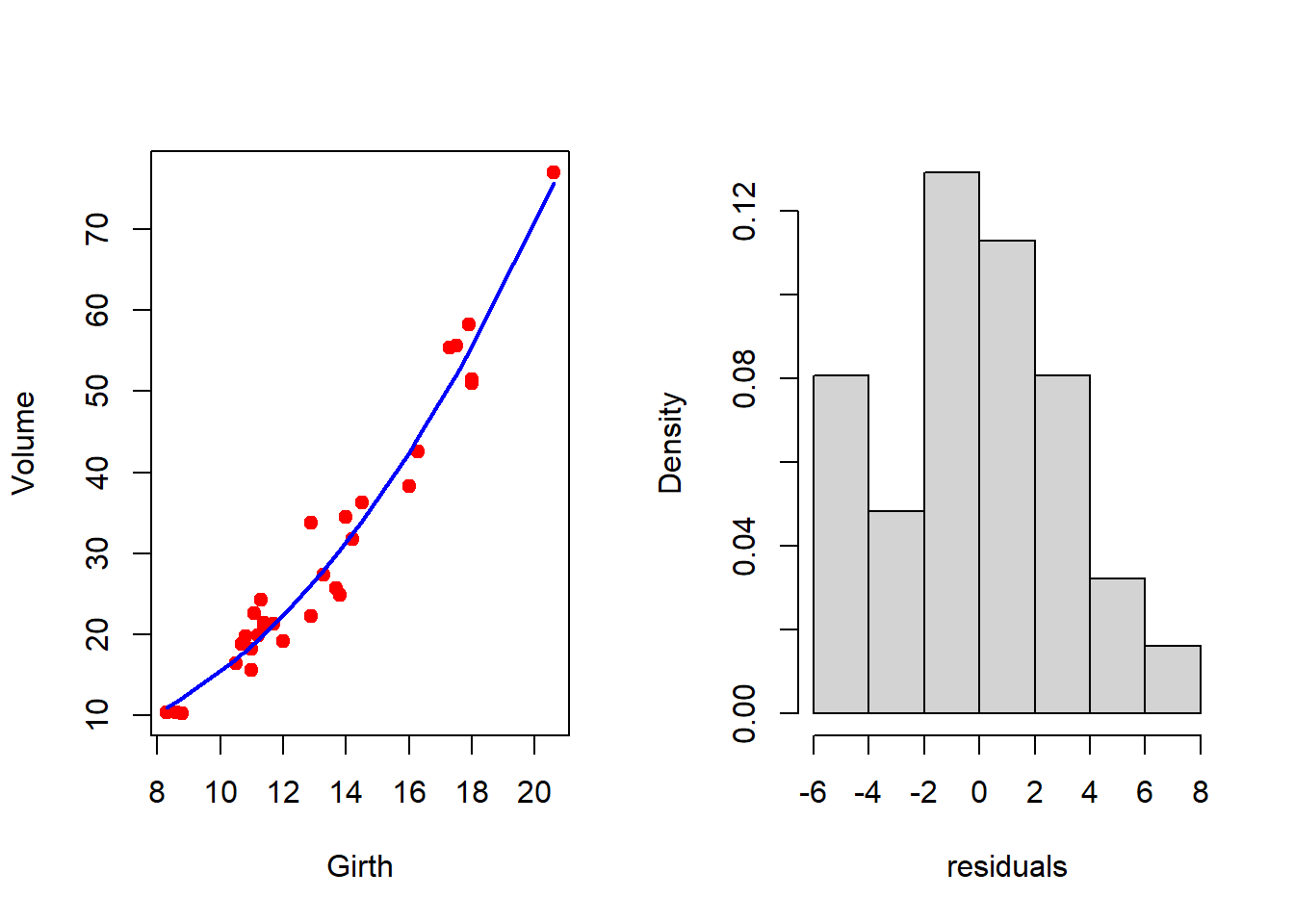
par(mfrow = c(2,2))
plot(fit2, col = "blue", pch = 19, lwd = 2)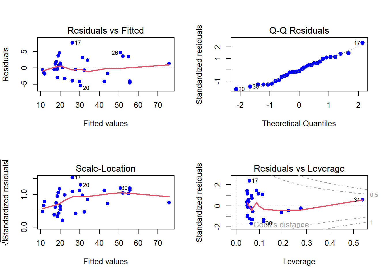
Now basically we have two statistical models. A natural question arises, whether making the mode complex, that is, considering quadratic from the linear regression, we have gained significantly or not. R provides a simple way of comparing two fitting exercises.
anova(fit, fit2)Analysis of Variance Table
Model 1: Volume ~ Girth
Model 2: Volume ~ Girth + I(Girth^2)
Res.Df RSS Df Sum of Sq F Pr(>F)
1 29 524.30
2 28 311.38 1 212.92 19.146 0.0001524 ***
---
Signif. codes: 0 '***' 0.001 '**' 0.01 '*' 0.05 '.' 0.1 ' ' 1The null hypothesis of the anova() function is that both the model performs equally well. However, from the obtained p-value of the output, the null hypothesis is rejected (very small p-value, ***).
14.2.2 Prediction and Confidence intervals
We go back to our original regression object fit (the simple linear regression) for discussing the difference between prediction and the confidence interval. Suppose we want to predict the volume of the timber for a new tree whose measurement of the diameter of the tree is provided and we plan to use the equation
\[\widehat{\text{Volume}} = \hat{\beta_0} + \hat{\beta_1}\times \text{Girth}.\]
It is an important task to report the uncertainty associated with the prediction. The variance associated with the prediction can be obtained by using the following formula:
\[Var(\widehat{\mbox{Volume}}) = Var(\hat{\beta_0}) + Var(\hat{\beta_1})\times \text{Girth}^2 + 2\times \text{Girth}\times Cov\left(\hat{\beta_0}, \hat{\beta_1} \right).\]
In the above, we have just applied the commonly known formula
\[Var(aX + bY) = a^2 Var(X) + b^2 Var(Y) + 2ab \times Cov(X, Y).\]
In the following we obtain the estimate of the Volume of timber as 59.30781 cubic ft for the tree having diameter of 19 inches with standard error of the estimate as 1.614811 cubic ft. Run the following code and understand the prediction interval is wider than the confidence interval.
new = data.frame(Girth = c(19))
predict(fit, newdata = new, se.fit = TRUE)
$fit
1
59.30781
$se.fit
[1] 1.614811
$df
[1] 29
$residual.scale
[1] 4.251988predict(fit, newdata = new, interval = "prediction") fit lwr upr
1 59.30781 50.0055 68.61013predict(fit, newdata = new, interval = "confidence") fit lwr upr
1 59.30781 56.00515 62.61047We first plot the prediction and the confidence intervals in the same plot and observe that the prediction intervals are wider than the confidence intervals. The reason is that the prediction intervals account for the randomness in the error component as well as the estimates in the systematic component. The confidence interval only considers the variation in \(\hat{\beta_0}\) and \(\hat{\beta_1}\), not the variance of \(\hat{\epsilon}\). Therefore, for prediction interval the variance of the prediction is computed as:
\[\begin{align} Var(\widehat{\mbox{Volume}}) & = Var(\hat{\beta_0} + \hat{\beta_1}\times \text{Girth} + \hat{\epsilon})\\ &= Var(\hat{\beta_0}) + Var(\hat{\beta_1})\times\text{Girth}^2 + 2\times \text{Girth}\times Cov\left(\hat{\beta_0}, \hat{\beta_1}\right) + Var(\hat{\epsilon}). \end{align}\]
The presence of an extra component \(Var(\hat{\epsilon})\) is evident from the calculations.
par(mfrow = c(1,1))
plot(Volume ~ Girth, data = trees, cex.lab = 1.2,
     col = "red", pch = 19, ylim = c(0, 80))
new = data.frame(Girth = seq(8, 22, by = 0.5))
pred_interval = predict(fit, newdata = new,
                        interval = "prediction")    # prediction
conf_interval = predict(fit, newdata = new,
                        interval = "confidence")    # confidence
lines(new$Girth, pred_interval[,2], col = "magenta",
      lwd = 2, lty = 2)
lines(new$Girth, pred_interval[,3], col = "magenta",
      lwd = 2, lty = 2)

lines(new$Girth, conf_interval[,2], col = "blue",
      lwd = 2, lty = 2)
lines(new$Girth, conf_interval[,3], col = "blue",
      lwd = 2, lty = 2)
legend("topleft", legend = c("Prediction Interval",
                             "Confidence Interval"),
       col = c("magenta", "blue"), lwd = c(2,2),
       lty = c(2,2), bty = "n")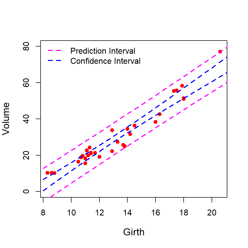
14.2.3 Incorporating other covariates
Till now we have discussed the regression model with a single predictor. However, there is another predictor Height (in ft) is also there. Suppose that we are now interested in including this covariate in modelling the Volume of timber using the following multiple linear regression model:
\[\mbox{Volume} = \beta_0 + \beta_1\times \text{Girth} + \beta_2\times \text{Height} + \epsilon\]{$eq-trees_MLR}
Using the lm() function in R, we can perform the fitting exercises and subsequently perform the regression diagnostics. The formula Volume ~ Girth + Height is understood as a multiple linear regression model by the lm() function.
fit3 = lm(formula = Volume ~ Girth + Height, data = trees)
summary(fit3)                       # summary of MLR
Call:
lm(formula = Volume ~ Girth + Height, data = trees)

Residuals:
    Min      1Q  Median      3Q     Max
-6.4065 -2.6493 -0.2876  2.2003  8.4847

Coefficients:
            Estimate Std. Error t value Pr(>|t|)
(Intercept) -57.9877     8.6382  -6.713 2.75e-07 ***
Girth         4.7082     0.2643  17.816  < 2e-16 ***
Height        0.3393     0.1302   2.607   0.0145 *
---
Signif. codes:  0 '***' 0.001 '**' 0.01 '*' 0.05 '.' 0.1 ' ' 1

Residual standard error: 3.882 on 28 degrees of freedom
Multiple R-squared:  0.948, Adjusted R-squared:  0.9442
F-statistic:   255 on 2 and 28 DF,  p-value: < 2.2e-16
Note that addition of another predictor gives the multiple R-squared value approximately \(95\%\), that is, we have obtained approximately \(1\%\). Using the anova() function, we can check whether this increment is significant or not.
anova(fit, fit3)Analysis of Variance Table
Model 1: Volume ~ Girth
Model 2: Volume ~ Girth + Height
Res.Df RSS Df Sum of Sq F Pr(>F)
1 29 524.30
2 28 421.92 1 102.38 6.7943 0.01449 *
---
Signif. codes: 0 '***' 0.001 '**' 0.01 '*' 0.05 '.' 0.1 ' ' 1The ANOVA table suggests only a marginal improvement is obtained by adding an extra covariate in the model. Such decisions are very important in the analysis of field data and must be reported with proper explanation. Often it is cited as the Art of Data Analysis, rather than the Science of Data Analysis.
In this case, the fitted regression function will be a plane instead of a line. In the following, we write a small piece of codes, that will plot of the regression plane. The persp() function in R is useful to draw three dimensional plots.
Girth_vals = seq(min(trees$Girth)-2,
                 max(trees$Girth)+2, by = 1)
Height_vals = seq(min(trees$Height)-2,
                  max(trees$Height)+2, by = 1)
fit3_vals = matrix(data = NA, nrow = length(Girth_vals),
                   ncol = length(Height_vals))
for(i in 1:length(Girth_vals)){
  for(j in 1:length(Height_vals)){
    fit3_vals[i,j] = coef(fit3)[1] + coef(fit3)[2]*Girth_vals[i] + coef(fit3)[3]*Height_vals[j]
  }
}                                               # Computation of predicted values
par(mfrow = c(1,1))
persp(Girth_vals, Height_vals, fit3_vals,
      col = "grey", xlab = "Girth", ylab = "Height",
      zlab = "Volume", theta = 10, cex.lab = 1.3)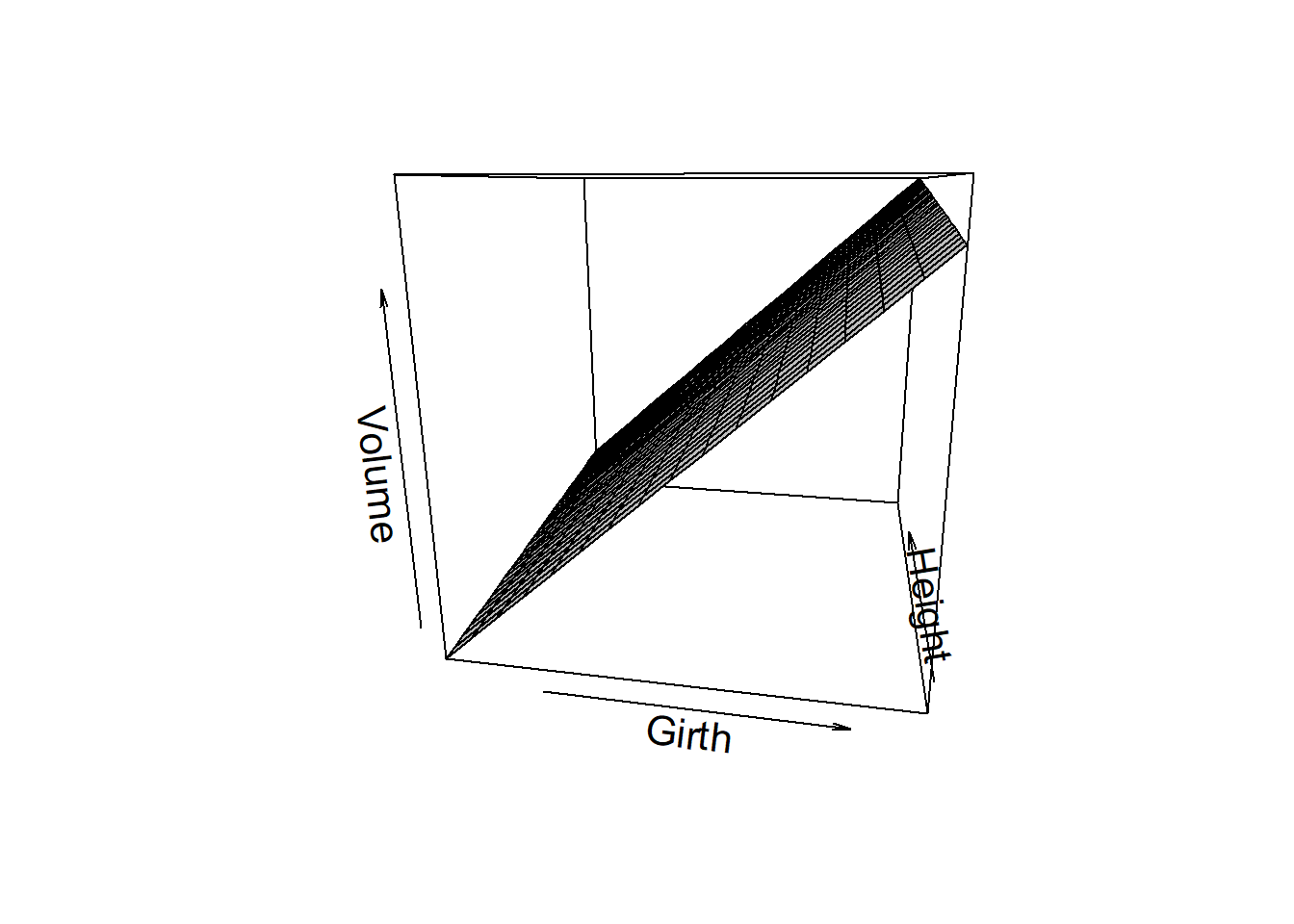
However, we can use plot3D package to generate nice plots. The colour gradients of the regression plane shade important light about the contribution of the predictors in the variation of the response variable.
library(plot3D)
persp3D(Girth_vals, Height_vals, fit3_vals,
        xlab = "Girth", ylab = "Height",
        zlab = "Volume", theta = 40, cex.lab = 1.3,
        alpha = 0.2)
points3D(trees$Girth, trees$Height, trees$Volume,
         col = "black", pch = 19, add = TRUE)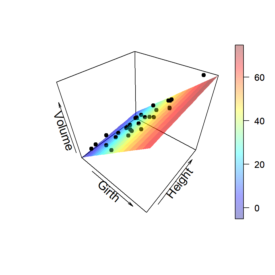
Using the package scatterplot3d, we can have interesting three dimensional visualization. The participants are encouraged to see the help file of the function scatterplot3d().
library(scatterplot3d)
scatterplot3d(trees$Girth, trees$Height, trees$Volume,
              xlab = "Girth (inches)",
              ylab = "Height (ft)", zlab = "Volume (cubic ft)",
              pch = 19, cex.lab = 1.2)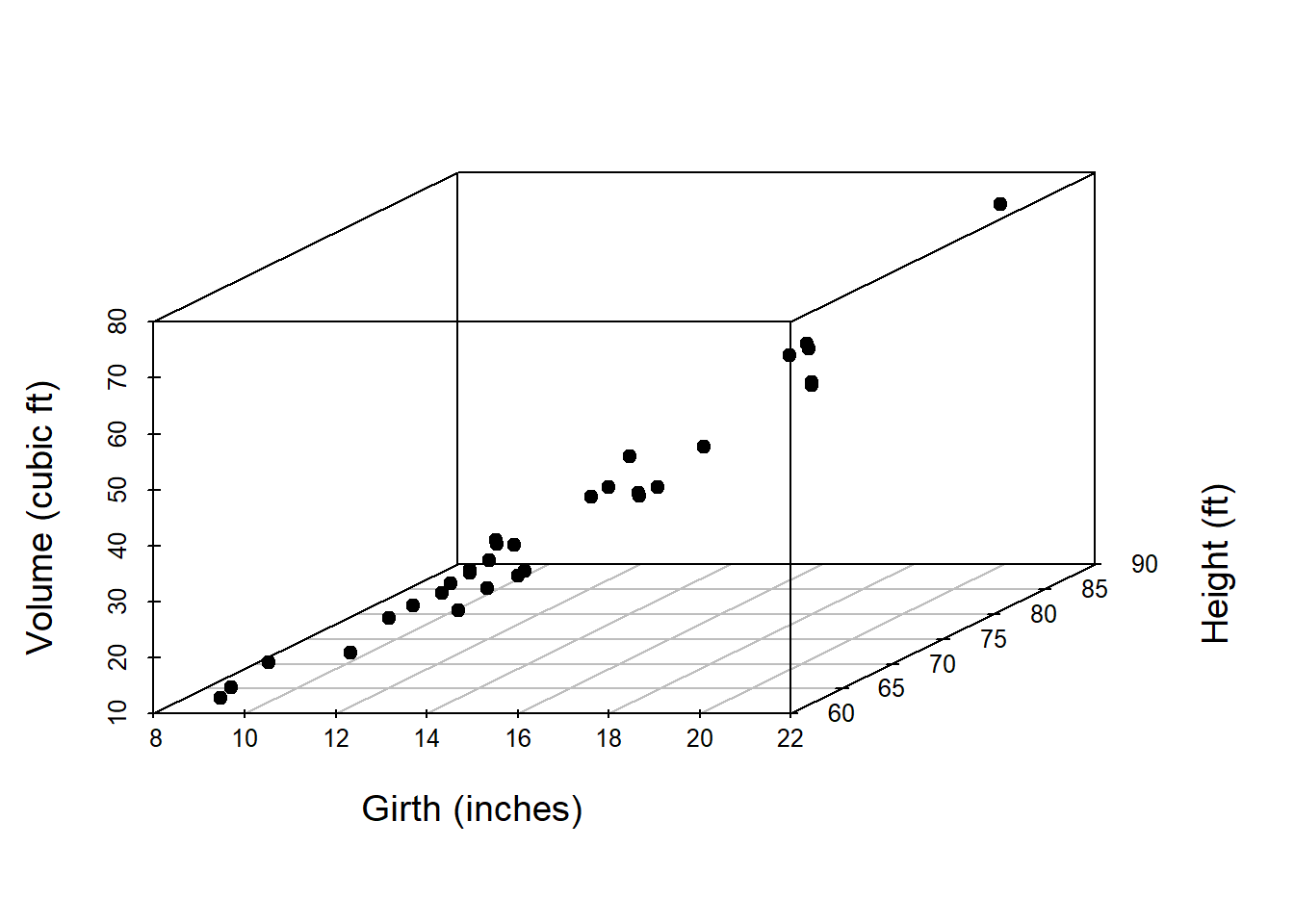
14.2.4 Impact of outliers in a regression model
There are some interesting functions in R which helps us to identify the influential points and leverage points in the regression model.
par(mfrow = c(1,2))
cooks.distance(fit)                                  # computing Cook’s distance
1 2 3 4 5 6
1.098362e-01 4.924417e-02 2.223564e-02 4.160457e-05 3.971050e-03 6.044249e-03
7 8 9 10 11 12
1.528743e-02 5.099320e-04 1.602747e-02 1.583849e-05 2.080153e-02 4.922094e-05
13 14 15 16 17 18
4.656599e-04 1.278988e-03 2.524848e-02 3.718828e-02 2.809168e-02 8.762270e-03
19 20 21 22 23 24
4.450995e-02 6.408063e-02 2.754799e-04 1.137428e-02 5.014444e-05 6.088904e-02
25 26 27 28 29 30
1.847520e-02 6.459356e-02 5.008387e-02 7.597544e-02 2.844384e-02 3.976321e-02
31
8.880581e-01 plot(cooks.distance(fit), pch = 19, col = "red",
cex.lab = 1.3, main = "Cook's Distance",
cex.main = 1.3) # plot the distance per obs
plot(Volume ~ Girth, data = trees, col = "red",
pch = 19, cex.lab = 1.3, main = "Fitted Lines",
cex.main = 1.3)
abline(fit, col = "blue", lwd = 2) # adding the fitted line
fit4 = lm(formula = Volume ~ Girth, data = trees[-31,])
abline(fit4, col = "magenta", lwd = 2) # fit without outlier
legend("topleft", legend = c("with 31", "without"),
col = c("blue", "magenta"), lwd = c(2,2), bty = "n")
points(trees$Girth[31], trees$Volume[31], col = "magenta",
cex = 2, lwd = 3) # mark the outlier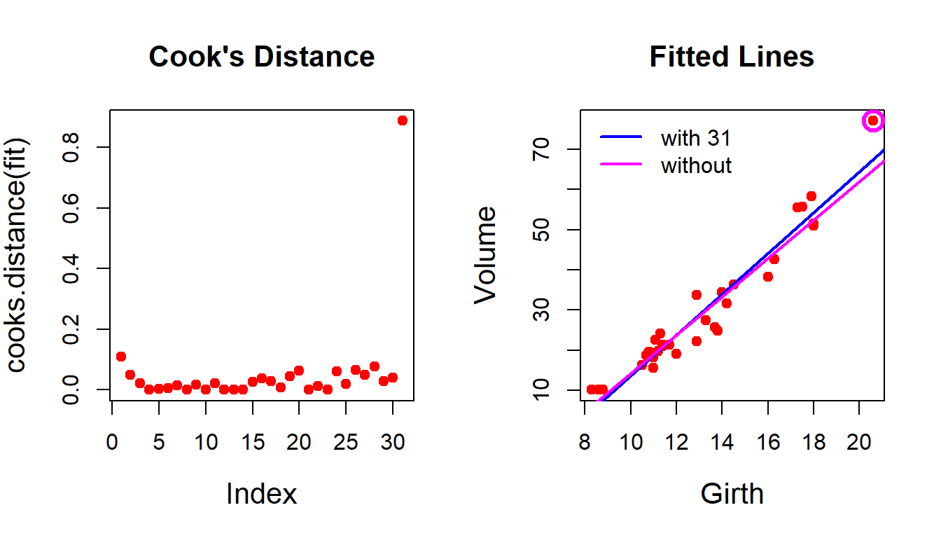
14.3 Universality of the normal distribution
We recollect the example of estimating the true probability of the success (\(p\)) from the coin tossing experiment. If we toss the coin n times and compute the proportion of success (\(\hat{p_n}\)). We keep the suffix \(n\) just to remind us that the distribution of the proportion of success changes as \(n\) changes.
- Suppose we fix \(n\) (the sample size) and simulate n coin tossing experiment using R with fixed success probability \(p=0.3\).
- We repeat this process \(M=1000\) times. In each repetition, we store the value of the proportion of success.
- From the step (b) we have \(M=1000\) many proportions of success (possibly different values).
- Draw a histogram of the values obtained in the previous steps.
- Repeat (a) – (d) for different choices of \(n\).
In the following, we implement the above steps. Let us remind ourselves that we are dealing with a coin tossing experiment and there is no discussion of normal distribution yet. One can envision the above simulation experiment as involving one thousand volunteers each tossing identical coins \(n\) times and reporting the proportion of successes. Intuitively, these proportions will vary due to inherent randomness. Our goal is to determine if this randomness can be described by a known probability distribution.
par(mfrow = c(2,3))
p = 0.3                                            # true P(success)
n_vals = c(5, 10, 20, 50, 100, 500)                # sample size
M = 1000                                           # number of replications
for(n in n_vals){                                  # loop of sample size
  p_hat = numeric(length = M)
  for(i in 1:M){                                   # loop on replications
    x = rbinom(n = n, size = 1, prob = p)
    p_hat[i] = sum(x)/n                            # sample proportion
  }
  hist(p_hat, probability = TRUE, main = paste("n = ", n),
       xlab = expression(widehat(p[n])), cex.lab = 1.3,
       cex.main = 1.3)
}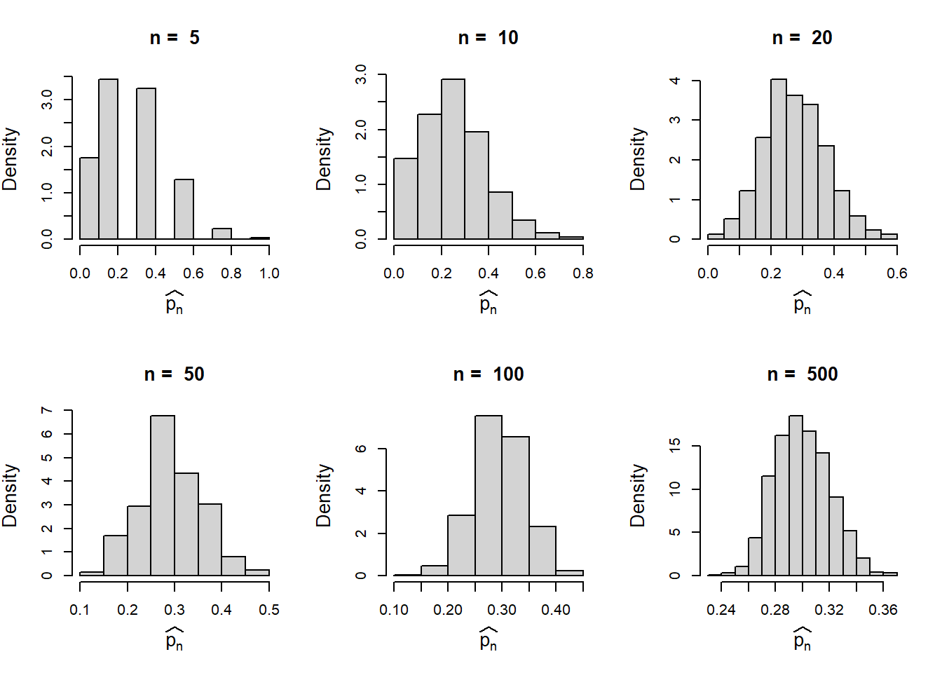
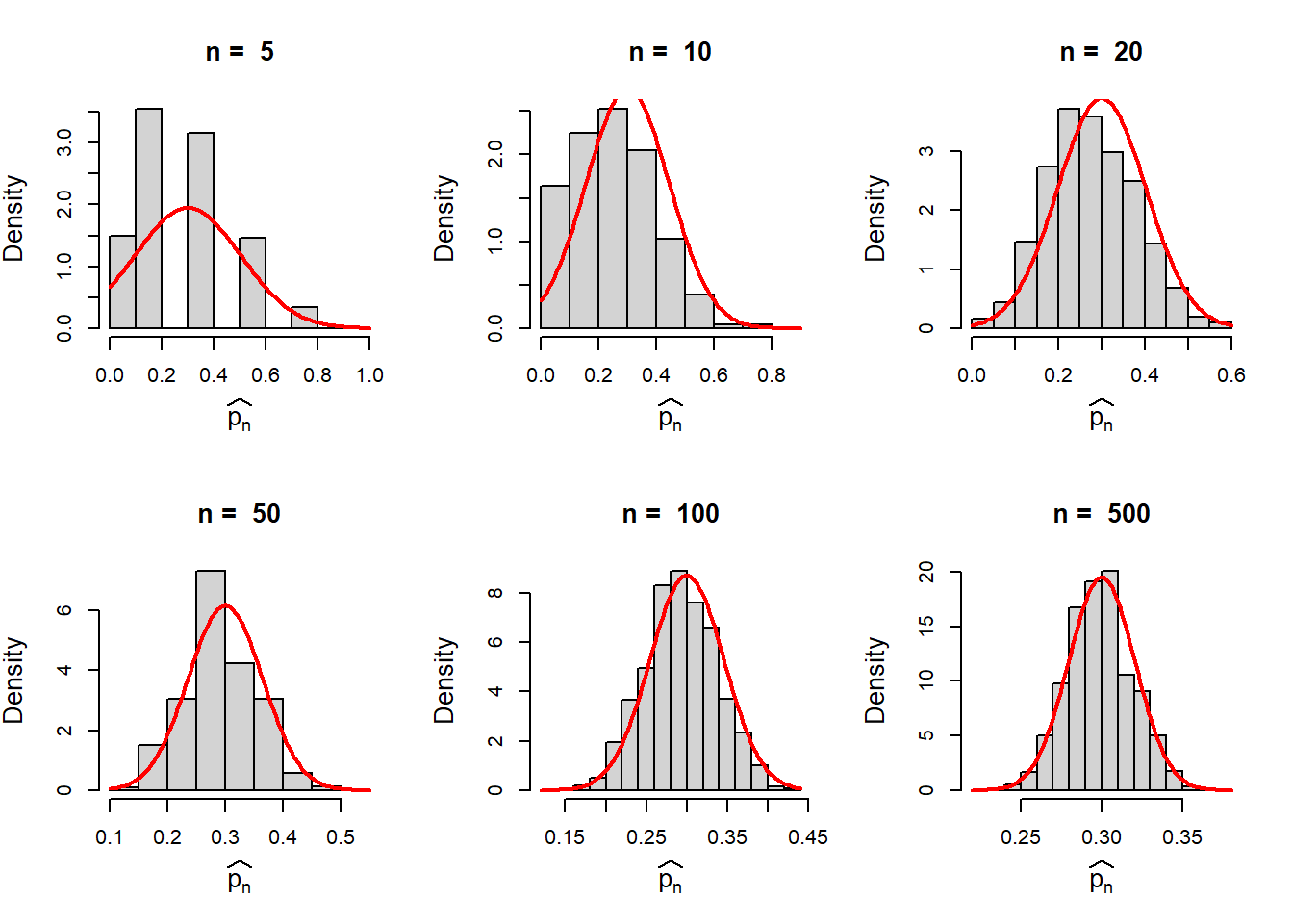
In the above simulation experiments, we observed that the histograms are centred about the true value \(p=0.3\). Let us compute the variance. Although, we do not belong to the statistics background, but simple basic calculations will help us to become better quantitative ecologists. For example, here, we want to compute \(Var(\hat{p_n})\).
First recall that if a random variable \(X\) takes only two values \(1\) or \(0\) with probability \(p\) and \(1-p\) respectively. Then the expectation of the random variable \(X\), denoted by \(E(X)\) is computed as follows:
\[\mbox{E}(X) = 0\times \mbox{P}(X=0) + 1\times \mbox{P}(X=1) = p.\] Therefore, empirically, we can say that from a single through of a coin, we can expect p many successes. This statement makes much more sense, when we say that if we toss the coin \(10\) times, approximately, the number of successes will be 10p. In other words, the proportion of successes in \(10\) repetitions of coin tossing experiment will be close to \(p\). The variance of \(X\) is computed as follows:
\[Var(X) = E(X^2) - (E(X))^2 = 0^2 \times P(X=0) + 1^2 \times P(X=1) - p^2 = p-p^2 = p(1-p).\]
We can think of the outcome of each coin tossing experiment as a random variable taking values either \(1\) or \(0\). Let \(X_1, \cdots, X_n\) be the outcome of the \(n\) coin tossing experiment and \(P(X=1) = P(\text{Head}) = p\). Therefore, the number of successes is \(X_1+ X_2+ \cdots+ X_n\) and outcome \(X_1\) does not impact \(X_2\) and similar for all the pairs.
\[Var(\hat{p_n}) = Var\left(\frac{X_1+ X_2+ \cdots+ X_n}{n}\right) = \frac{1}{n^2}\sum_{i=1}^{n}Var(X_i) = \frac{1}{n^2}\sum_{i=1}^{n}p(1-p) = \frac{p(1-p)}{n}.\]
Therefore, the standard error of \(\hat{p_n}\) is
\[\mbox{SE}(\widehat{p_n}) = \sqrt\frac{p(1-p)}{n}.\]
In the previous code snippet, we overlay each of the histogram with the normal density function with mean \(p\) and standard deviation \(\sqrt\frac{p(1-p)}{n}\).
par(mfrow = c(2,3))
p = 0.3
n_vals = c(5, 10, 20, 50, 100, 500)            # sample size
M = 1000                                       # number of replications
for(n in n_vals){
  p_hat = numeric(length = M)
  for(i in 1:M){
    x = rbinom(n = n, size = 1, prob = p)
    p_hat[i] = sum(x)/n
  }
  hist(p_hat, probability = TRUE, main = paste("n = ", n),
       xlab = expression(widehat(p[n])), cex.lab = 1.3,
       cex.main = 1.3)
  curve(dnorm(x, mean = p, sd = sqrt(p*(1-p)/n)),
        add = TRUE, col = "red", lwd = 2)       # add normal PDF
}
The reader is encouraged to perform the above experiment for other distributions as well, like Poisson(\(\lambda\)), Geometric(\(p\)), Exponential(\(\beta\)), Gamma(\(\alpha, \beta\)), Beta(\(a,b\)), etc. The letter r will be used for simulation purposes for all the distributions.
To summarize, basically, \(\hat{p_n}\) is an average of the outcomes \(X_i\)’s and the randomness in the average values can be well approximated by the normal distribution. This is due to the well-known Central Limit Theorem which states that the sample mean is well approximated by the normal distribution for large sample size \(n\).
For the reader, we repeat this experiment using the exponential distribution with parameter \(\beta=1\). The exponential distribution with mean \(\beta\) is given by
\[f(x) = \begin{cases} \frac{1}{\beta}e^{-\frac{x}{\beta}},~0<x<\infty\\ 0,~~~~\text{Otherwise}. \end{cases}\]
The curve function can be conveniently used to draw the exponential PDF for different values of \(\beta\). In the following, we plot three PDF side by side for \(\beta \in\{1,2,0.5\}\).
par(mfrow = c(1,3))
curve(dexp(x, rate = 1), col = "red", -1, 6,
      lwd = 2, main = expression(paste(beta, " = ", 1)),
      cex.main = 1.4, cex.lab = 1.3)
curve(dexp(x, rate = 2), col = "red", -1, 4,
      lwd = 2, main = expression(paste(beta, " = ", 2)),
      cex.main = 1.4, cex.lab = 1.3)
curve(dexp(x, rate = 0.5), col = "red", -1, 10,
      lwd = 2, main = expression(paste(beta, " = ", 0.5)),
      cex.main = 1.4, cex.lab = 1.3)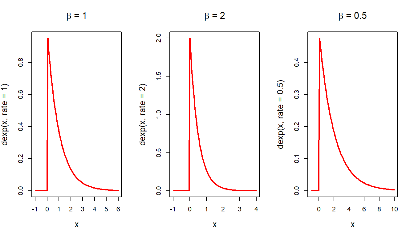
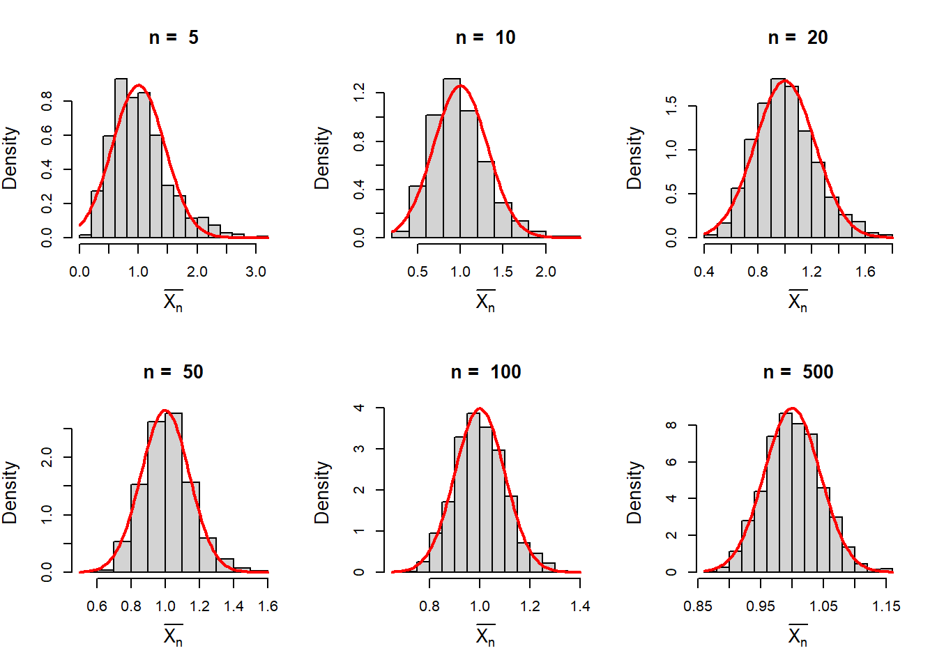
Now suppose that we draw a random sample of size n from the exponential distribution with \(\beta=1\). The mean of the distribution is \(\beta\). The sample mean \(\frac{1}{n}\sum_{i=1}^{n}X_i = \bar{X_n}\) can be well approximated by the normal distribution. In the following, we see that the histograms are bell shaped for large \(n\) values.
par(mfrow = c(2,3))
beta = 1
n_vals = c(5, 10, 20, 50, 100, 500) # sample size
M = 1000                            # number of replications
for(n in n_vals){
  sample_means = numeric(length = M)
  for(i in 1:M){
    x = rexp(n = n, rate = 1/beta)
    sample_means[i] = sum(x)/n
  }
  hist(sample_means, probability = TRUE, main = paste("n = ", n),
       xlab = expression(bar(X[n])), cex.lab = 1.3,
       cex.main = 1.3)
  curve(dnorm(x, mean = beta, sd = beta/sqrt(n)),
        add = TRUE, col = "red", lwd = 2)
}
14.4 Nonlinear Regression Models
In the investigations of natural processes, many times we come across nonlinear relationships between the response and the predictors. We have already discussed some aspects of linear regression using R particularly the use of the function lm() in R. This function is particularly useful for the linear models or nonlinear models which can be converted to a linear model. However, there are many models that cannot be written as a linear function of the parameters. In such a case, nonlinear regression modelling is required. In R the nls() function takes care of the estimation of parameters for nonlinear function.
To investigate the nonlinear regression concepts in the context of ecological models, we first describe a phenomenon known as the Allee effect. The Allee effect, named after ecologist W. C. Allee, corresponds to density-mediated drop in the population fitness when they are small in numbers (Allee, 1931; Dennis, 1989; Fowler and Baker, 1991; Stephens and Sutherland, 1999). The harmful effects of inbreeding depression, mate limitation, predator satiation etc. reduce fitness as the population size decreases. For such dynamics, the maximum fitness is achieved by the species at an intermediate population size, unlike logistic or theta-logistic growth models. Such observations usually correspond to the mechanisms giving rise to an Allee effect. In recent decades, due to an increasing number of threatened and endangered species, the Allee effect has received much attention from conservation biologists. The related theoretical consequences and the empirical evidence have made the Allee effect an important component in both theoretical and applied ecology. In general, there are two types of Allee effects are considered in the natural populations across a variety of taxonomic groups, viz. component and demographic Allee effect. The component Allee effect modifies some component of individual fitness with the changes in population sizes or density. If the per capita growth rate is low at small density but remains positive is called the weak demographic Allee effect. The strong Allee effect is characterized by a threshold density below which the per capita growth rate is negative that leads to extinction deterministically. The critical density is called the Allee threshold and has significant importance in conservation biology (Hackney and McGraw, 2001), population management (Myers et al., 1995; Liermann and Hilborn, 1997) and invasion control (Johnson et al., 2006). There are a large number of studies available in the literature on the mathematical modelling of the demographic Allee effect (see Table 3.1 Courchamp et al. (2008)).
A bit of mathematical quantities to measure the growth of populations would be helpful to understand the context. If \(X(t)\) represents the population size at time \(t\), then, the derivative of the population size with respect to \(t\), that is \(\frac{dX(t)}{dt}\) is called the absolute growth rate and \(\frac{1}{X(t)}\frac{dX(t)}{dt}\) is called the per capita growth rate (PGR) at time t. Note the that the PGR has dimension \(\text{time}^{-1}\). If rate of growth is bigger than zero, then the population grows and if it is negative population decline.
Consider the following equation
\[\frac{dX}{dt} = rX\left(\frac{X}{A}-1\right)\left(1-\frac{X}{K}\right), ~X(0) = X_0.\]
The quantities \(A\) is the Allee threshold and \(K\) is the carrying capacity of the environment and \(r\) is the intrinsic growth rate. The parameters \(A\) and \(K\) satisfy the inequality \(0<A<K\). It is easy to see that if \(X_0<A\), then \(\frac{dX}{dt}<0\), that means the population declines and for \(0<X_0<K, \frac{dX}{dt}>0\), therefore, the population grows.
In the following we learn how to solve such differential equations using R. Then, we can visualize various dynamics of the population with various initial population sizes \(X_0\).
library(deSolve)                           # load the library
A = 30                                     # Allee threshold
K = 80;                                    # Carrying capacity
AlleeFun = function(t, state, param){      # Allee growth equation
  with(as.list(c(state,param)),{
    dX = r*X*(X/A - 1)*(1 - X/K);
    return(list(c(dX)));
  })
}
parameters = c(r = 0.5, K = 80,A = 30)     # parameters of the model
times = seq(0, 10, by = 0.01)              # time frame
init.pop = 35                              # initial population size
state = c(X = init.pop)
out = ode(y = state, times = times, func = AlleeFun,
          parms = parameters)              # solving the ODE
plot(out, main = "Solution of Allee growth equation",
     ylim=c(10, 90), xlab = "time",
     ylab = "population size", col = 2, lwd = 2,
     cex.lab = 1.3)
abline(h = A, col = 6, lwd=2, lty=2)       # horizontal line at A
abline(h = K, col = 8, lwd=2, lty=3)       # horizontal line at K
text(0, 83, "K", lwd = 2)
text(0, 33, "A", lwd = 2)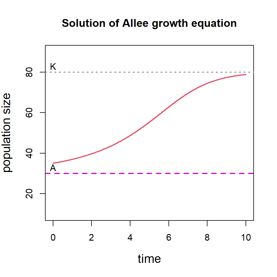
We can consider multiple initial population size and see how the solution of the differential equation behaves. The following code will show that if the initial population size is below threshold \(A\), the population goes to extinction and if the initial population size is above \(A\), the population eventually settles down at \(K\).
init.pop = c(10, 20, 40, 50, 60, 100)        # Different initial size
for(i in 1:length(init.pop)){
  state = c(X = init.pop[i])
  out = ode(y = state, times = times, func = AlleeFun,
            parms = parameters)
  if(i==1)
    plot(out, main = "Solution of Allee growth equation",
         ylim=c(0, 100), xlab = "time",
         ylab = "population size", col = i, lwd = 2,
         cex.lab = 1.3)
  else
    lines(out, col = i, lwd = 2)
}
abline(h = A, col = 6, lwd=2, lty=2)
abline(h = K, col = 8, lwd=2, lty=3)
text(0, 83, "K", lwd = 2)
text(0, 33, "A", lwd = 2)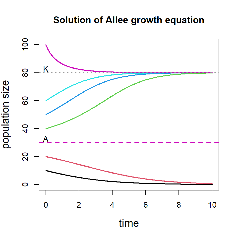
14.4.1 Fitting of the Allee growth equations
Before going into fitting exercises, we shall learn how to simulate the population dynamics from the model populations. Suppose that we want to simulate the population dynamics of a population governed by the Allee growth equation and the population is subject to demographic stochasticity alone.
First, we fix the parameters for the simulations. We simulation the initial population size \(X_0\sim N(25,3^2 )\) and the simulate the per capita growth from \(r_t\sim \mathcal{N}(\mu_t,\sigma^2 dt)\), where \(\mu_t=r\left(\frac{X_t}{A}-1\right)\left(1-\frac{X_t}{K}\right)\). Then we simulate \(X_1\sim X_0 e^{r_t dt}\). The process is continued till the end time point. In the following code, we first fix the parameters:
r = 0.05                                   # true parameter value r
A = 20                                     # Allee threshold
K = 100                                    # Carrying capacity
time = seq(0, 10, by = 0.05)               # time points
dt = time[2] - time[1]                     # time difference
sig_e = 0.1                                # environmental standard deviation
par(mfrow = c(1,2))
In the following code, we perform a single simulation of the population dynamics.
popSim = numeric(length = length(time))
x0 = rnorm(n = 1, mean = 30, sd = 3)
popSim[1] = x0
for (i in 1:(length(time)-1)) {
  mu = r*(popSim[i]/A - 1)*(1- popSim[i]/K)
  pgr = rnorm(n = 1, mean = mu, sd = sig_e*sqrt(dt))
  popSim[i+1] = popSim[i]*exp(pgr)
}
plot(time, popSim, col = "red", lwd = 2, type = "l",
     xlab = "time", ylab = "Population size", cex.lab = 1.3)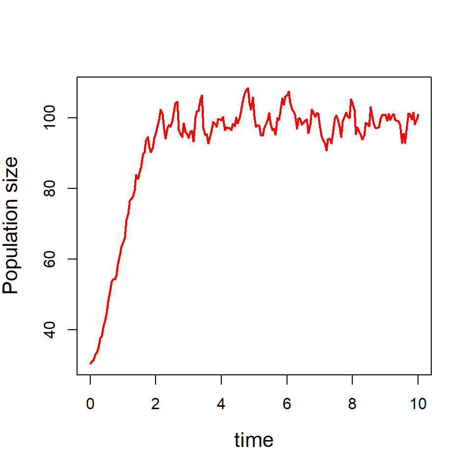
In the following we perform 50 simulations and obtain 50 possible population trajectories.
nsim = 50
popSim = matrix(data = NA, nrow = nsim, ncol = length(time))
popSim = matrix(data = NA, nrow = nsim, ncol = length(time))
for(i in 1:nsim){
  x0 = rnorm(n = 1, mean = 25, sd = 5)
  popSim[i,1] = x0
  for (j in 1:(length(time)-1)) {
    mu = r*(popSim[i,j]/A - 1)*(1- popSim[i,j]/K)
    pgr = rnorm(n = 1, mean = mu, sd = sig_e*sqrt(dt))
    popSim[i, j+1] = popSim[i,j]*exp(pgr)
  }
}
matplot(time, t(popSim), type = "l", lty = 1,
        ylab = "Population size", cex.lab = 1.3)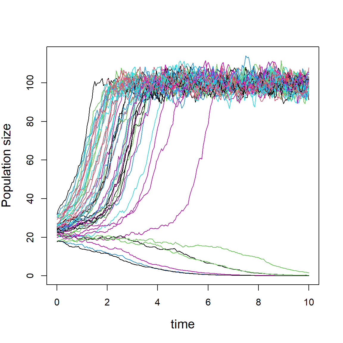
Now we concentrate on the fitting of the Allee growth equation to the real data set. Suppose that the following data has been collected from the field of some species populations.
29, 30, 31, 32, 34, 37, 40, 42, 43, 45, 52, 59, 61, 54, 58, 63, 65, 71, 74, 75, 77, 82, 83, 89, 91, 97, 95, 105, 97, 102, 104, 99, 101, 95, 100, 97, 98, 100, 102, 98, 97.
First, we store these data values in an object \(x\) using the concatenation operator \(c\) and then plot both size profile and time per capita growth profile of the population. We estimate the per capita growth
par(mfrow = c(1,2))
x = c(29, 30, 31, 32, 34, 37, 40, 42, 43, 45, 52, 59, 61, 54, 58, 63,
      65, 71, 74, 75, 77, 82, 83, 89, 91, 97, 95, 105, 97, 102, 104,
      99, 101, 95, 100, 97, 98, 100, 102, 98, 97)
plot(x, type = "b", pch = 19, col = "red",
     xlab = "Years", ylab = "Population size", cex.lab = 1.2)
n = length(x)                                       # length of the data
R = log(x[2:n]/x[1:(n-1)])                          # Per capita growth rate
plot(x[1:(n-1)], R, xlim = c(0, 120), col = "grey",
     ylab = "PGR", xlab = "Population size", pch = 19,
     cex.lab = 1.2)
abline(h = 0, col = "red", lwd = 2)                 # adding horizontal line

nls_fit = nls(R ~ r*(x[1:(n-1)]/A-1)*(1-x[1:(n-1)]/K),
              start = list(r = 0.04, A= 20,K=90))
summary(nls_fit)                                    # summary of the nls
Formula: R ~ r * (x[1:(n - 1)]/A - 1) * (1 - x[1:(n - 1)]/K)

Parameters:
  Estimate Std. Error t value Pr(>|t|)
r  0.01018    0.06629   0.154    0.879
A  3.83204   22.88810   0.167    0.868
K 98.61951    4.36712  22.582   <2e-16 ***
---
Signif. codes:  0 '***' 0.001 '**' 0.01 '*' 0.05 '.' 0.1 ' ' 1

Residual standard error: 0.04698 on 37 degrees of freedom

Number of iterations to convergence: 5
Achieved convergence tolerance: 4.522e-08
r_hat = coefficients(nls_fit)[1] # estimate of r
A_hat = coefficients(nls_fit)[2] # estimate of A
K_hat = coefficients(nls_fit)[3] # estimate of K
curve(r_hat*(x/A_hat-1)*(1-x/K_hat), add = TRUE,
col = "blue", lwd = 2) # adding fitted curve
Similar to the linear regression, nonlinear regression models can also be compared. Suppose that the same per capita growth profile is also analysed using the logistic growth equation. The logistic growth equation is given by
\[\frac{dX}{dt} = r_m X\left(1-\frac{X}{K}\right), ~ X(0) = X_0, \tag{14.3}\] where, \(r_m\) is the intrinsic growth rate (also referred to as the maximum per capita growth rate) and \(K\) is the carrying capacity of the environment. Add the following code snippet below the previous code snippet.
Here, the per capita growth profile of the logistic growth equation is a linear function of the population size \(r_m \left(1-\frac{X}{K}\right)\) which can be written in the form \(a+bX\), where \(a=r_m\) and \(b=-\frac{r_m}{K}\). Therefore, we can apply linear regression model to perform this fitting exercise, however, we apply the nls() function only to get the estimates of \(r_m\) and \(K\) as given below. Therefore, nls() function can also be used to perform linear regression.
plot(x[1:(n-1)], R, xlim = c(0, 120), col = "grey",
     ylab = "PGR", xlab = "Population size", pch = 19,
     cex.lab = 1.2)
abline(h = 0, col = "red", lwd = 2)                     # adding horizontal line
curve(r_hat*(x/A_hat-1)*(1-x/K_hat), add = TRUE,
      col = "blue", lwd = 2)                            # adding fitted curve

nls_fit_log = nls(R ~ r_m*(1-x[1:(n-1)]/K),
                  start = list(r_m = 0.04, K=90))       # fitting of logistic
rm_hat = coefficients(nls_fit_log)[1]                   # estimate of rm
K_hat = coefficients(nls_fit_log)[2]                    # estimate of K
curve(rm_hat*(1-x/K_hat), add = TRUE,
      col = "magenta", lwd = 2)                         # add fitted curve
legend("bottomleft", legend = c("Allee growth", "Logistic"),
       col = c("blue", "magenta"), lwd = c(2,2),
       bty = "n", cex = c(0.8, 0.8))                    # add legend to plot
In the following, we compare the curve fitting exercises. One way to look at the actual versus predicted values and a high correlation between them gives indication of a better fitting. In the following, we plot the actual and fitted per capita growth rates obtained by Allee growth equation and the logistic growth equation. We also compute the corresponding correlations.
par(mfrow = c(1,2))
plot(R, fitted.values(nls_fit), pch = 19, col = "grey",
     xlab = "Observed PGR", ylab = "Fitted PGR", cex.lab = 1.2,
     main = "Allee growth equation")
cor(R, fitted.values(nls_fit))                     # correlation value
[1] 0.5125905abline(lm(fitted.values(nls_fit) ~R), col = "red", lwd = 2)
plot(R, fitted.values(nls_fit_log), pch = 19, col = "grey",
xlab = "Observed PGR", ylab = "Fitted PGR", cex.lab = 1.2,
main = "Logistic growth equation") # R versus fitted values
abline(lm(fitted.values(nls_fit_log) ~R), col = "red", lwd = 2)
cor(R, fitted.values(nls_fit_log)) # correlation value[1] 0.4515992
For the Allee and logistic growth model fitting, the correlation between the observed per capita growth rate and predicted per capita growth rates are \(0.51\) and \(0.45\), respectively, which shows approximately \(50\%\) agreement. Using the AIC function, we also compute the Akaike Information Criterion to compare these two fitting exercises.
AIC(nls_fit)[1] -126.2541AIC(nls_fit_log)[1] -125.1844The difference between the AIC values is less than \(5\), therefore, these two models perform almost in a similar way.
Till now, in our discussion, we have considered the all the data points. It is important to note that one data point always lie away from the mass of the per capita growth rate values. In the scatterplot of actual versus fitted values, in the top left corner of the window, a data point is observed. As a practitioner, presence of such points needs to be considered and take appropriate action. This will be an exercise for the participants to redo the above exercises by fitting exercises without this stipulated point which is suspected to be an outlier.
14.5 Bootstrapping regression model
Bootstrapping is a powerful resampling technique which helps in evaluating the goodness of the fitting exercises. In the bootstrapping process, we create a new data set from the original data set. We have the data set which contains the first column as the population size and the second column as the per capita growth rates at those population sizes. If there are n rows in the data, we randomly select n rows from the data following the principle of simple random sampling with replacement (SRSWR) and create a new data set with those selected rows. It is understood that in the new data set some rows may be repeated (due to SRSWR). The new data set is called the bootstrap data set. We create \(B=1000\) bootstrap data sets from the original data set. We perform the fitting exercise on each of the bootstrap data sets and record the estimates of the parameters. The histogram of the \(B\) many estimates constitute the bootstrap sampling distribution of the estimators of the parameters. We carry out this exercise for the logistic growth model using the above data set.
B = 1000                                       # number of bootstrap samples
rm_hat = numeric(B)                            # bootstrap estimate of rm
K_hat = numeric(B)                             # bootstrap estimate of K

D = data.frame(R = R, x = x[1:(n-1)])          # original data
for(i in 1:B){
  ind = sample(1:nrow(D), replace = TRUE)      # SRSWR
  nls_fit_boot = nls(R ~ r_m*(1-x/K), data = D[ind,],
                     start = list(r_m = 0.1, K = 80))
  rm_hat[i] = coefficients(nls_fit_boot)[1]    # bootstrap estimate
  K_hat[i] = coefficients(nls_fit_boot)[2]     # bootstrap estimate
}
par(mfrow = c(1,2))
hist(rm_hat, probability = TRUE, main = "",
     xlab = expression(widehat(r[m])), breaks = 30)
hist(K_hat, probability = TRUE, main = "",
     xlab = expression(widehat(K)), breaks = 30)
The reader is encouraged to update the above code and compute the AIC values for each of the bootstrap fitting. If the bootstrap distribution of the AIC values is wide, which indicates the sensitivity of the fitting on the individual data points.
14.6 Some more concepts in Model selection
Let us get back to our data analysis task once again. We tried to predict the volume of the timber using the Girth variable as the predictor. In fact, we ended up with two regression models one is linear, and the other one is quadratic. We can predict the volume for some diameter of a tree for whom the volume is not available. A natural question arises, how would we validate the predictions, that is, how close the predictions to the true volume of the timer? One may argue that future is always unknown, therefore, there is no chance to check the goodness of the predictions. Or in other words, we need to rely completely on the model that is built on the whole data set (here there are 31 rows).
14.6.1 Training and test set
We may think of having a better strategy. Our whole data set consists of 31 rows, and we can keep about \(20\%\) of the rows aside (about 6 rows) and build the models on rest \(80\%\) of the rows. In the data science literature, the bigger set (\(80\%\)) on which the model fitting exercises are carried out, is called the training data. The smaller set is referred to as the test data. The fitted model is used to predict the volume of timber using the girth values in the test data. It is important to note that the predicted values on the test data can now be assessed how close they are to the actual response values. The selection of the training data (rows) is done randomly, that is, randomly 25 rows are selected out of the 31 rows and create a training data consisting of the selected 25 rows and we create another data set with remaining 6 rows. In this new setting we minimize the following sum of squares and obtain the estimates of the parameters \(b_0, b_1\) and \(σ^2\):
\[ \sum_{i=1}^{25}\left(\text{Volume}_i^* - b_0-b_1\times\text{Girth}_i^*\right)^2.\] And we predict the volume on the test data using \(\text{Volume}_i = b_0+b_1\times\text{Girth}_i\), where \(i\) represents the rows in the data which belongs to the test set. The test set contains six observations. Therefore, we have six predictions of the volume. The accuracy of the predictions is assessed by the mean squared error as follows:
\[\frac{1}{6}\sum_{i=1}^{6}\left(\widehat{\text{Volume}_i}-\text{Volume}_i\right)^2.\] The above quantity gives an idea how good the predictions are and also referred to as test mean squared error (mse). In fact, this can be used to compare the prediction accuracy for two different models. The same exercise can be carried out for the quadratic regression model as well. If the prediction accuracy for the quadratic regression is more than the linear regression model, one may prefer to utilize the quadratic equation for the prediction purpose. Performing the train-test procedure is essentially to provide a greater confidence level that the fitted model expected to perform well on the future observation.
Let us execute the above task and check the predictive accuracy of the linear and quadratic regression model to predict the volume of the timber using the diameter. The following R code will do this task. We will use the sample function to select 25 rows randomly out of 31 rows in the data set.
data(trees)
train = sample(1:nrow(trees), size = floor(nrow(trees)*0.8))
train_trees = trees[train, ]                                 # training data
print(train)                                                 # training rows
test_trees = trees[-train, ]                                 # test data
train_fit = lm(Volume ~ Girth, data = train_trees)
train_fit2 = lm(Volume ~ Girth + I(Girth^2),
                data = train_trees)
predict_fit = predict(train_fit, newdata = test_trees)
predict_fit2 = predict(train_fit2, newdata = test_trees)

mean((predict_fit - test_trees$Volume)^2)                    # test mse linear
mean((predict_fit2 - test_trees$Volume)^2)                   # test mse quadratic
The reader is encouraged to run above code snippet multiple times and observe the test mean squared error values change in different runs. This is due to the random selection of the rows. Using the print(train) you can check which rows are being selected in the training data.
To come to an objective conclusion, we should not deal with such type of randomness, and we seek to get a measure that takes care of this randomness. The test mean squared error is a random quantity. We may seek to compute the average test mean squared error. The idea is that we perform the train test process a large number of times (\(M\), say) and every time compute the test mean squared error and compute the average error. The quadratic model will be preferred if the average test mean squared error is less than the average test mean squared error for the simple linear regression model. Let us do this task below and compute the average test mean squared error for both the models.
M = 500                                    # number of repetitions
test_mse_fit = numeric(length = M)         # store test mse linear
test_mse_fit2 = numeric(length = M)        # store test mse quadratic
for(i in 1:M){
  train = sample(1:nrow(trees), size = floor(nrow(trees)*0.8))
  train_trees = trees[train, ]             # training data
  test_trees = trees[-train, ]             # test data
  train_fit = lm(Volume ~ Girth, data = train_trees)
  train_fit2 = lm(Volume ~ Girth + I(Girth^2),
                  data = train_trees)
  predict_fit = predict(train_fit, newdata = test_trees)
  predict_fit2 = predict(train_fit2, newdata = test_trees)
  test_mse_fit[i] = mean((predict_fit - test_trees$Volume)^2)
  test_mse_fit2[i] = mean((predict_fit2 - test_trees$Volume)^2)
}
par(mfrow = c(1,2))                                     # two plots side by side
hist(test_mse_fit, probability = TRUE,
     main = "Linear Regresion", breaks = 30,
     xlab = "test mse", cex.lab = 1.3)            # distribution of test mse
points(mean(test_mse_fit), 0, pch = 19,
       col = "red", cex = 1.3)                      # average test mse
hist(test_mse_fit2, probability = TRUE,
     main = "Quadratic Regression", breaks = 30,
     xlab = "test mse", cex.lab = 1.3)
points(mean(test_mse_fit2), 0, pch = 19,
       col = "red", cex = 1.3)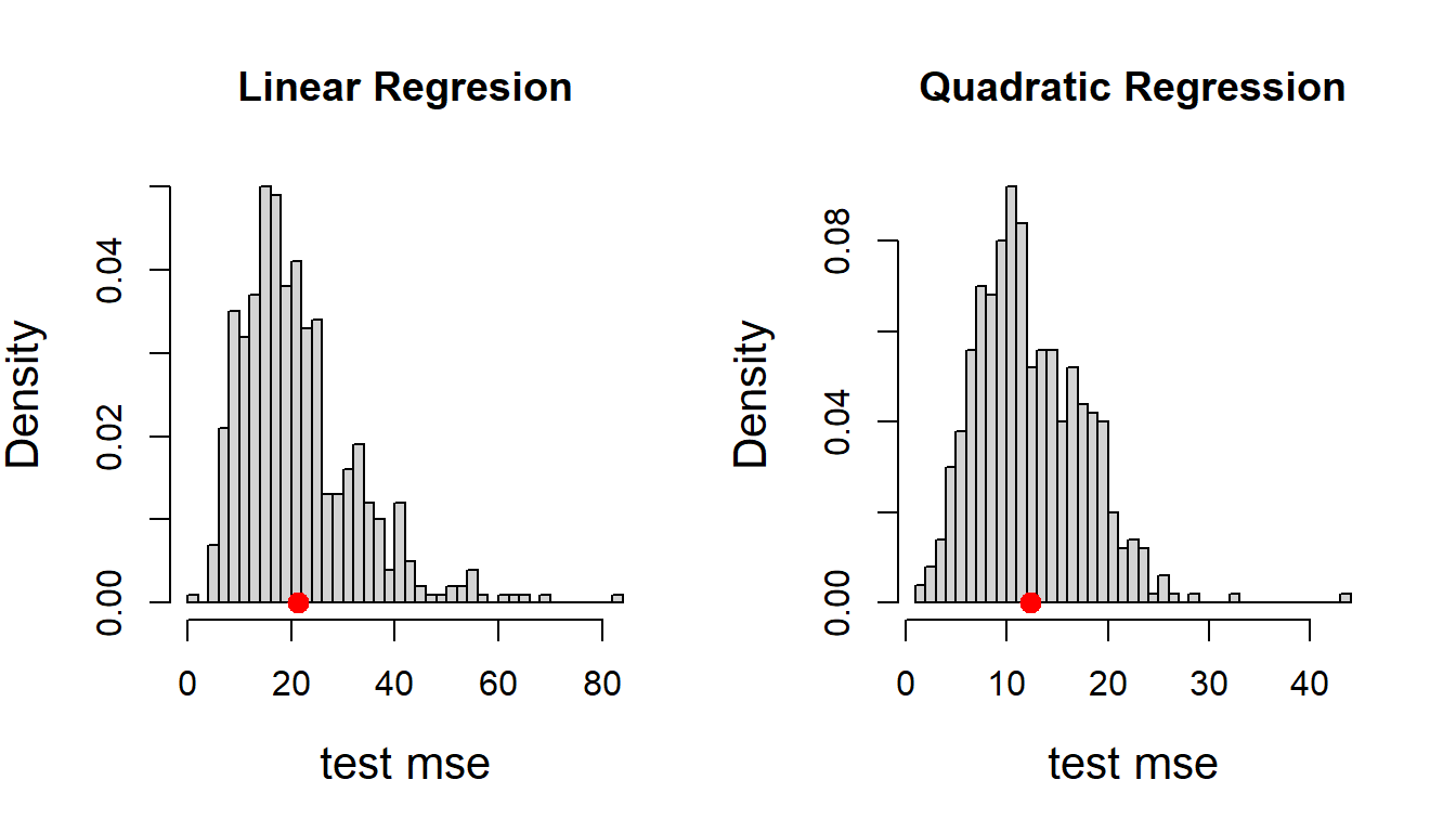
One may argue that by this process it is not guaranteed that all the individual data points has been used as a training point or as test point. Therefore, still some dependence on the individual data points remained. One way to deal with it to ensure that every row in the data set is a part of both training and test data. Suppose consider the first row as the test data and rest 30 rows as training data. Based on the fitted model we obtain the prediction for the first row and compute \(\left(\widehat{\text{Volume}_1}-\text{Volume}_1\right)^2\). The same process is carried out by removing the second row and compute \(\left(\widehat{\text{Volume}_2}-\text{Volume}_2\right)^2\) and continue this process till the \(31^\text{st}\) row. Basically, each data point is used as both training and test data point and this process is known as Leave One Out Cross Validation (LOOCV). The LOOCV error is computed as:
\[\frac{1}{31}\sum_{i=1}^{31}\left(\widehat{\text{Volume}_i}-\text{Volume}_i\right)^2.\] The model with the lesser LOOCV error may be preferred as the prediction equation for the given data analysis problem. In the following, let us compute the LOOCV error for both simple linear regression and quadratic regression model.
test_mse_fit = numeric(length = nrow(trees))
test_mse_fit2 = numeric(length = nrow(trees))
for(i in 1:nrow(trees)){
  train_trees = trees[-i, ]                            # drop ith the row
  test_trees = trees[i, ]                              # ith row in test
  train_fit = lm(Volume ~ Girth, data = train_trees)
  train_fit2 = lm(Volume ~ Girth + I(Girth^2),
                  data = train_trees)
  predict_fit = predict(train_fit, newdata = test_trees)
  predict_fit2 = predict(train_fit2, newdata = test_trees)
  test_mse_fit[i] = (predict_fit - test_trees$Volume)^2
  test_mse_fit2[i] = (predict_fit2 - test_trees$Volume)^2
}

cat("The LOOCV error of the linear regression model\n")
The LOOCV error of the linear regression modelmean(test_mse_fit) # LOOCV linear regression [1] 20.5653cat("The LOOCV error of the quadratic regression model\n")The LOOCV error of the quadratic regression modelmean(test_mse_fit2) # LOOCV quadratic regression[1] 11.93375The output of the above code gave the LOOCV estimate of the prediction error (test mean squared error) \(20.5652\) and \(11.93375\) for the linear and quadratic regression, respectively. Therefore, by using the leave one out cross validation, one may choose to go ahead with the quadratic regression model to predict the volume of the timber as a function of tree diameter. The reader is encouraged to implement the above piece of code for the model
\[\text{Volume} = b_0 + b_1 \times \text{Girth} + b_2 \times \text{Height} + \epsilon.\]
An important I would like to stress here that, whenever we run a regression model (here using the lm() function), many matrix multiplications take place at the background and there is computational task involved it. Sometimes, depending on the implementation of the algorithm, it may take longer time to run the codes. We observed that for implementation of the LOOCV, we had to execute the lm() function code 31 times, or in general, it is the number of rows in the data. Imagine that if there were \(10^5\) rows in the data with several predictors, running the code several times, would be extremely difficult task. Therefore, LOOCV may not always computationally handy.
Therefore, we need to devise some mechanism, by which we need to implement a smaller number of runs like train-test process and at the same time we can ensure that all the data points are ensured to be the part of both set of training and test observations. The method, called, K-fold validation ease this task. Suppose that we have data set with 100 rows, and we want to implement a five-fold cross validation. In this process, we divide the data into five approximately equal segments. Before writing the codes, we keep a note of the following points:
- LOOCV is a special case of the k-fold cross validation, where k is chosen to be equal to the number of observations.
- LOOCV is time consuming due the number of experiments performed, if the dataset is large enough.
- With k-fold cross-validation, the computation time is reduced due to the number of experiments performed is less as well as the all the observations are eventually used to train and test the model.
Similar to the LOOCV, one can write a simple for loop to execute the task. However, we will use a simple but useful package in R. We will use the caret package to complete this task. The function train() in the caret package offers several options for model training. In the trainConrol option, we specify the number of folds.
#install.packages("caret", dependencies = TRUE)
library(caret)                                       # load the library
out = train(Volume ~ Girth, data = trees,
            method = "lm",
            trControl = trainControl(method = "cv", number = 5))
print(out$results[2])                      # RMSE
RMSE
1 4.406795out2 = train(Volume ~ Girth + I(Girth^2), data = trees,
method = "lm",
trControl = trainControl(method = "cv", number = 5))
print(out2$results[2]) # RMSE RMSE
1 3.525031From the output it is found that the 5-fold cross validation root mean squared errors are \(4.45317\) and \(3.264002\) for the linear and quadratic regression, respectively. Therefore, by using the K-fold cross validation, we consider the quadratic regression model as a better predictive model for the volume of timber. We would like to emphasize that the choice of the folds is randomly done. Therefore, if we run the above code once again, the values might be changed. Therefore, we may repeat this process a certain number of times and report the average K-fold cross validation error and corresponding standard error value. This can be carried out by fixing the repeats option in the trainControl argument. In the following, we just provide the updated code:
out = train(Volume ~ Girth, data = trees,
            method = "lm",
            trControl = trainControl(method = "repeatedcv",
                                     number = 5, repeats = 100))
print(out$results[2])                  # linear regression
RMSE
1 4.366103cat("The estimated RMSE is ", as.numeric(out$results[2]),
" with standard error ", as.numeric(out$results[5]))The estimated RMSE is 4.366103 with standard error 1.159246out2 = train(Volume ~ Girth + I(Girth^2), data = trees,
method = "lm",
trControl = trainControl(method = "repeatedcv",
number = 5, repeats = 100))
print(out$results[2]) # quadratic regression RMSE
1 4.366103cat("The estimated RMSE is ", as.numeric(out2$results[2]),
" with standard error ", as.numeric(out2$results[5]))The estimated RMSE is 3.421973 with standard error 0.738747