In this tutorial, we shall understand how to fit nonlinear regression models using R for some give data set. We shall consider only a single input variable age and out variable size.
We shall first simulate the data set artificially with some fixed parameter choices and then apply nonlinear least squares on the data set. This will help us to understand the accuracy of the nonlinear least squares method using R.
12.2 Simulation of growth data
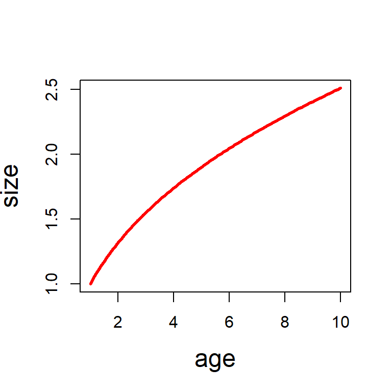
For demonstration we consider the following nonlinear function \[\mbox{size} = a\times \mbox{age}^b + \mbox{e}\] where \(a\) and \(b\) are fixed parameter and the error component \(\mbox{e}\) has normal distribution with mean \(0\) and variance \(\sigma^2\). We use the function \(\texttt{set.seed()}\) to ensure that the simulation studies are reproducible. For simulation study, we fixed the parameter values as \(a = 1\), \(b=0.4\) and \(\sigma = 0.2\).
set.seed(123)age =seq(1, 10, by =0.1) # age variableprint(age)
plot(age, size, type ="l", lwd =3, col ="red", cex.lab =1.5)
Figure 12.1: The mean growth profile. The parameters are fixed at \(a=1\) and \(b=0.4\). The plot should be considered as a conditional expectation of the \(\texttt{response variable}\) (size) at different values of age variable. \(\mbox{E}(\mbox{size}|\mbox{age})\) as a function of age. If we fixe age = 4 (say), then expected size is \(a\times 4^b\).
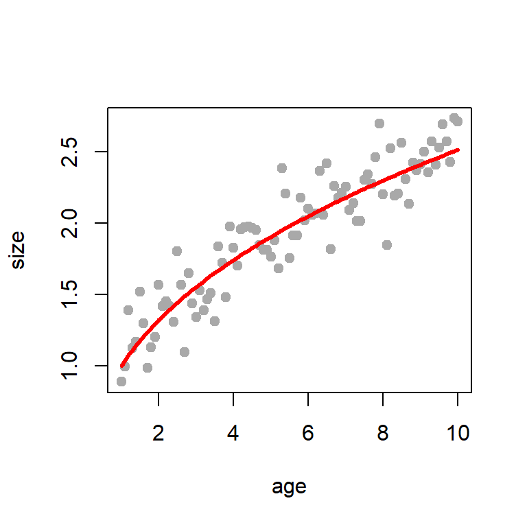
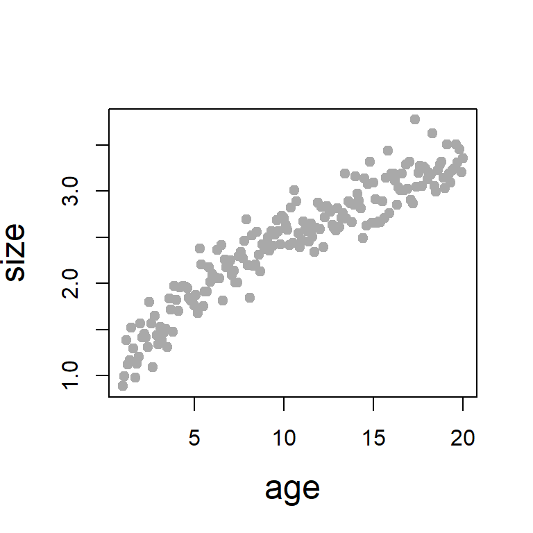
set.seed(123)size = a*age^b +rnorm(n =length(age), mean =0, sd =0.2)# print(size)plot(age, size, col ="darkgrey",pch =19)lines(age, a*age^b, col ="red", lwd =3)data =data.frame(age, size)head(data)
Figure 12.2: The simulated data set. The function set.seed() is set at 123 to ensure that the simulation study is reproducible. The parameters \(a = 1\), \(b=0.4\) and \(\sigma = 0.2\). The sample size is \(n = 91\). The true conditional mean value of the response given age is added in red colour.
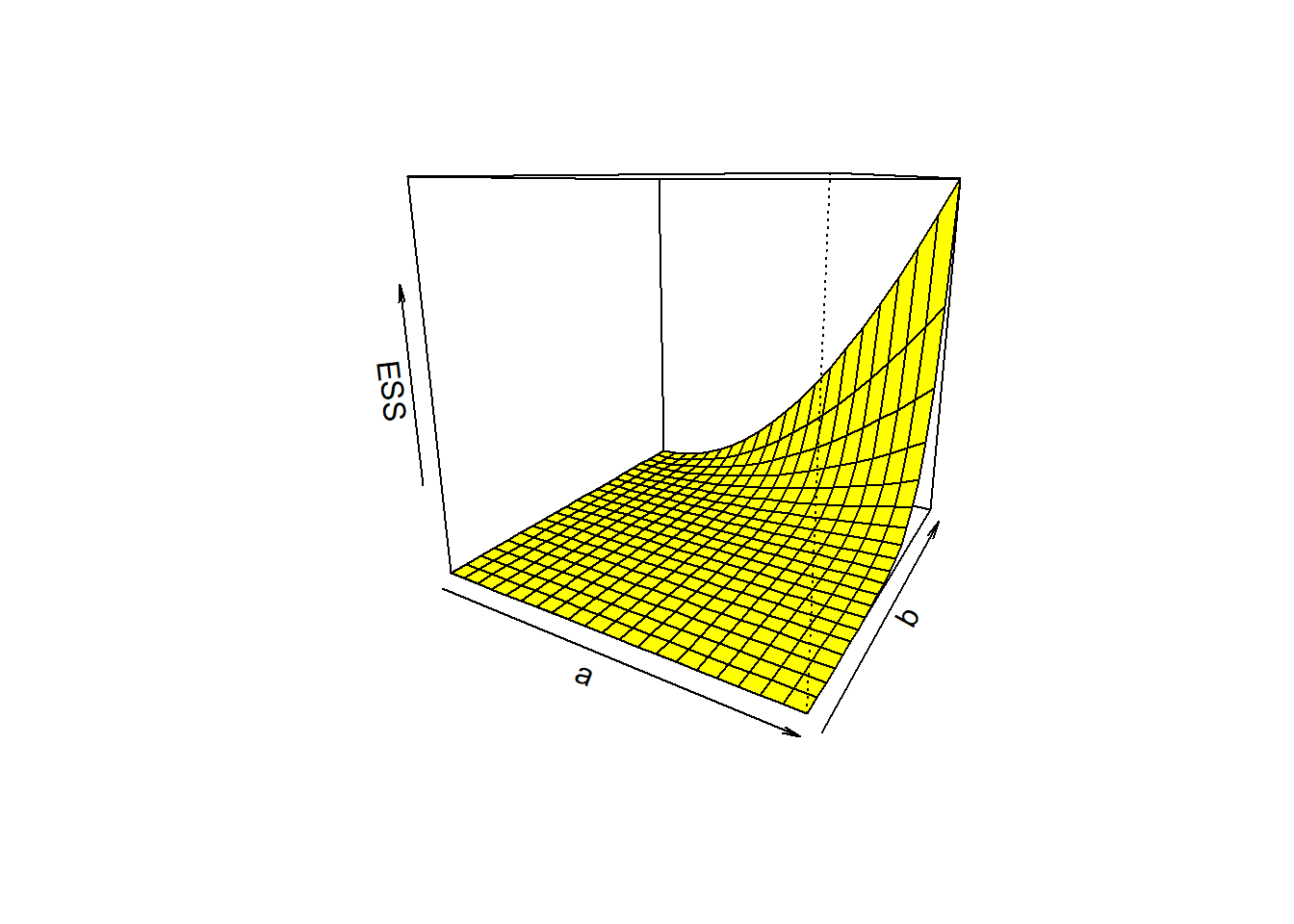
To estimate the parameters based using the simulated data, we need to minimize the error sum of squares which is given by \[\mbox{ESS} = \sum_{i=1}^n\left(\mbox{size}_i - a\times \mbox{age}_i^b\right)^2\] with respect to \(a\) and \(b\). In the following we try to visualize the \(\mbox{ESS}\) as a function of \(a\) and \(b\). \(n\) is the sample size or the number of rows in the data set.
ESS =function(a, b){ # Error sum of squaressum((size - a*age^b)^2)}a_vals =seq(0, 2, by =0.1)b_vals =seq(0, 2, by =0.1)ESS_vals =matrix(data =NA,nrow =length(a_vals),ncol =length(b_vals))for (i in1:length(a_vals)) {for (j in1:length(b_vals)) { ESS_vals[i,j] =ESS(a_vals[i], b_vals[j]) }}cat("The matrix containing the error sum of squares values:\n")
The matrix containing the error sum of squares values:
Figure 12.3: The variation of the error sum of squares as a function of \(a\) and \(b\). We need to choose the values of the parameters at which the surface is minimum.
12.3 nonlinear least squares using R
The function is used to perform to obtain the nonlinear least squares estimate of \(a\) and \(b\). To execute the nls function, we need to provide an initial starting point for the parameters.
fit =nls(size ~ a*age^b, data = data,start =list(a =0.5, b =1))coefficients(fit)
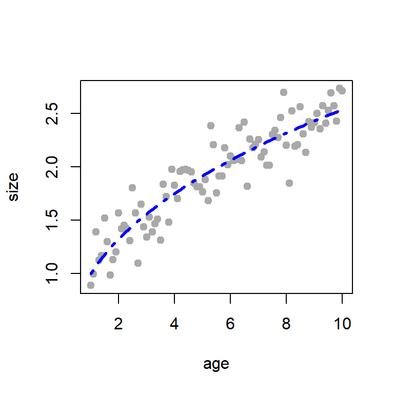
size_hat =fitted.values(fit) # store predicted valueserror_hat =residuals(fit)plot(age, size, pch =19, col ="darkgrey")lines(age, size_hat,col ="blue", lwd =3, lty =10)
Figure 12.4: The fitted allometric growth equation using the nls routine in R.
12.4 Some diagnostics
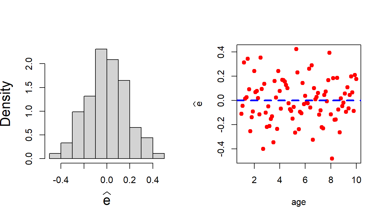
par(mfrow =c(1,2))hist(error_hat, probability =TRUE,xlab =expression(widehat(e)),cex.lab =1.5, main =" ")plot(age, error_hat, pch =19,col ="red", ylab =expression(widehat(e)))abline( h =0, col ="blue",lwd =3, lty =2)
Figure 12.5: The behaviour of the residuals play the most critical role in nonlinear regression models.
12.5 Understanding the summary of nls
The function allows to understand the uncertainty associated with the estimated parameters.
summary(fit)
Formula: size ~ a * age^b

Parameters:
  Estimate Std. Error t value Pr(>|t|)
a  0.99943    0.03719   26.88   <2e-16 ***
b  0.40405    0.02011   20.09   <2e-16 ***
---
Signif. codes:  0 '***' 0.001 '**' 0.01 '*' 0.05 '.' 0.1 ' ' 1

Residual standard error: 0.1795 on 89 degrees of freedom

Number of iterations to convergence: 4
Achieved convergence tolerance: 7.866e-06
AIC(fit)
[1] -50.38962
BIC(fit)
[1] -42.85704
12.6 Understanding the uncertainty of nls estimates
If we want to understand the uncertainty associated with the parameter estimates, we need to repeat the following process \(M\) times (say) and obtain \(M\) many estimates of \(a\) and \(b\). The histograms of these estimated values will give us an idea how the estimates will vary if we repeatedly sample data from the same model population. Let us repeat the above task here \(M=1000\) times and obtain the estimates \(\widehat{a}\) and \(\widehat{b}\) in each repetition.
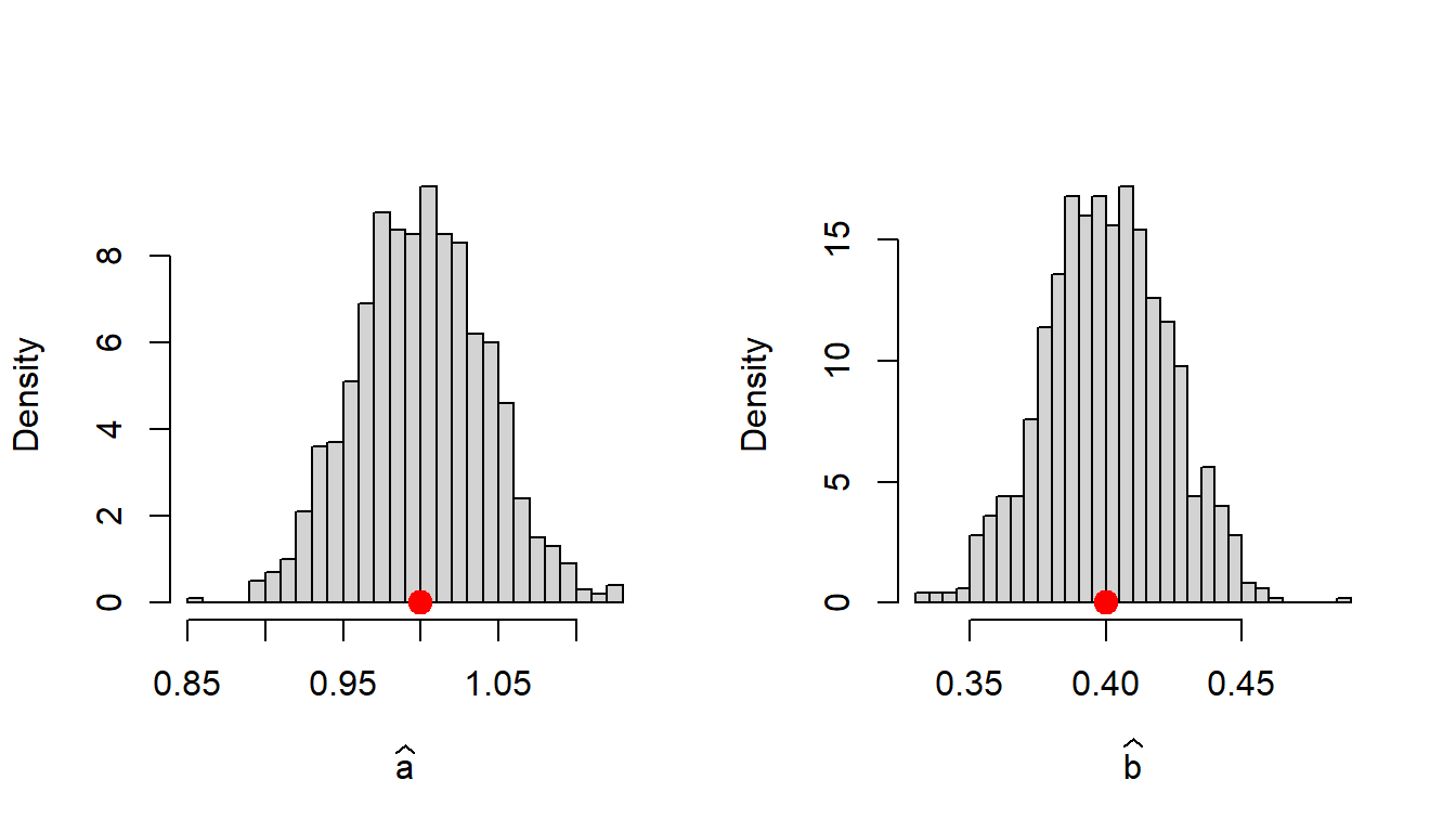
M =1000# number of repetitionsage =seq(1, 10, by =0.1) # age variablea =1# true value of ab =0.4# true value of ba_hat =numeric(length = M)b_hat =numeric(length = M)for (i in1:M) {set.seed(i) size = a*age^b +rnorm(n =length(age), mean =0, sd =0.2) data =data.frame(age, size) fit =nls(size ~ a*age^b, data = data,start =list(a =0.5, b =1)) a_hat[i] =coefficients(fit)[1] b_hat[i] =coefficients(fit)[2]}par(mfrow =c(1,2))hist(a_hat, probability =TRUE, xlab =expression(widehat(a)),main =" ", breaks =30)points(a, 0, pch =19, col ="red", cex =1.5)hist(b_hat, probability =TRUE, xlab =expression(widehat(b)),main =" ", breaks =30)points(b, 0, pch =19, col ="red", cex =1.5)
Figure 12.6: The approximate sampling distribution of the nonlinear least squares estimates of \(a\) and \(b\). The sampling distribution is quiet well approxiamted by the normal distribution. In addition, note that the estimated values are centered about the true values of \(a\) and \(b\) using which the articial data sets have been simulated.
12.7 Homoschedasticity versus heteroschedasticity
The statistical model to perform the nonlinear regression model is of the following form: \[\mbox{size}_i = a\times \mbox{age}_i^b + \mbox{e}_i,~i\in\{1,2,\ldots,n\}.\] In the previous simulations, we have consider that \(Var(\mbox{e}_i)=\sigma^2\) for all \(i\in \{1,2,\ldots,n\}\), that means, at different age, the variability in the size variable remains same about the true mean function. To simulate a scenario, we consider that \(Var(\mbox{e})= \sigma^2 \times \mbox{age}^2\). It means that as the age increases, the variability in size also increases.
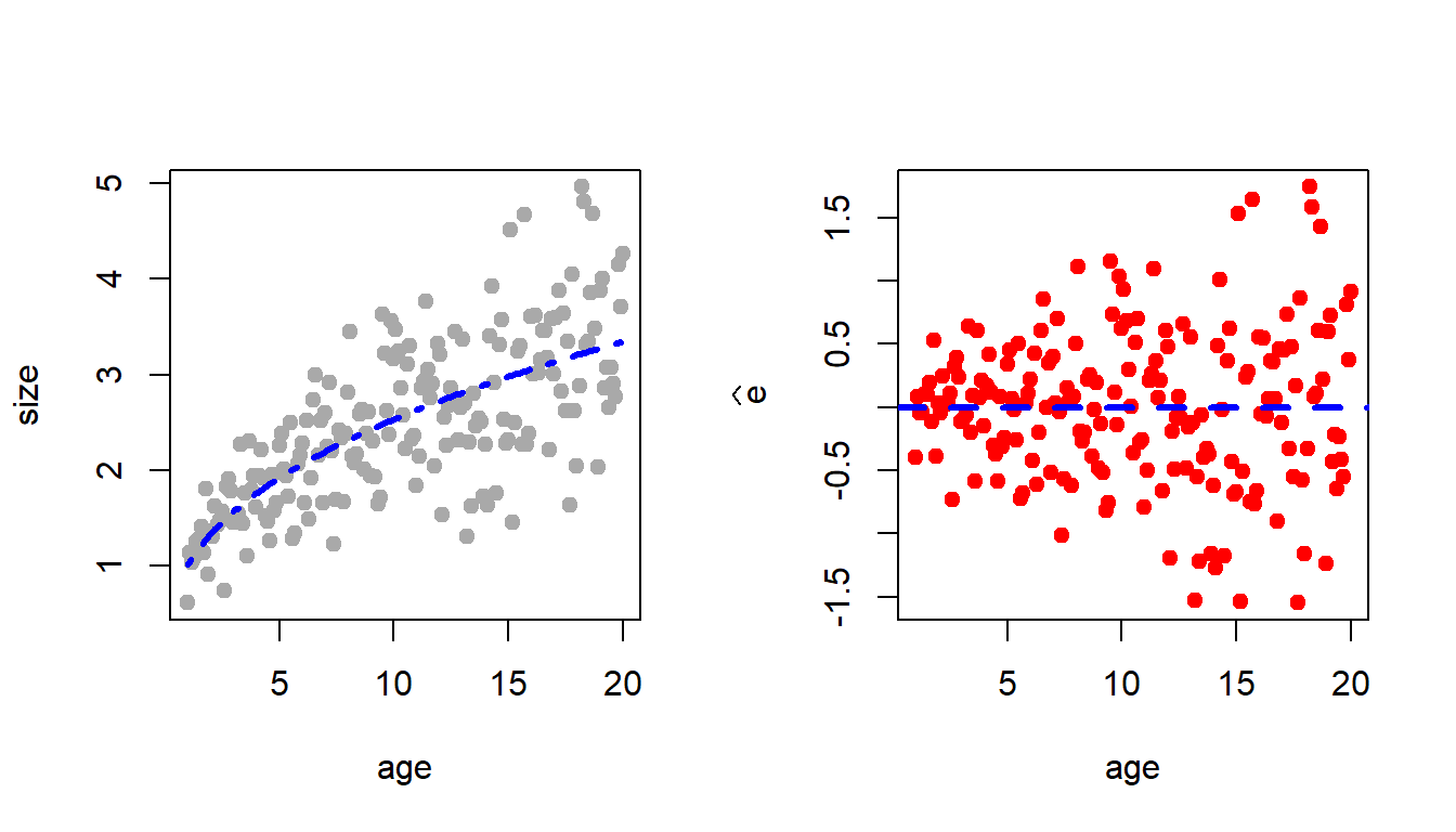
par(mfrow =c(1,2))a =1b =0.4age =seq(1, 20, by =0.1)size = a*age^b +rnorm(n =length(age), mean =0, sd =0.2*sqrt(age))data =data.frame(age, size)fit =nls(size ~ a*age^b, data = data,start =list(a =0.5, b =1))size_hat =fitted.values(fit) # store predicted valueserror_hat =residuals(fit)plot(age, size, pch =19, col ="darkgrey")lines(age, size_hat, col ="blue", lwd =3, lty =10)plot(age, error_hat, pch =19, col ="red", ylab =expression(widehat(e)))abline( h =0, col ="blue", lwd =3, lty =2)
Figure 12.7: The simulated data gives clear indication of the presence of heteroschedasticity. The plot of residuals against the age gives whether the errors do not have a constant variance.
12.8 Confidence Interval and Prediction Interval
a =1b =0.4age =seq(1, 20, by =0.1)size = a*age^b +rnorm(n =length(age), mean =0, sd =0.2)data =data.frame(age, size)fit =nls(size ~ a*age^b, data = data,start =list(a =0.5, b =1))
The nonlinear least squares estimates of \(a\) and \(b\) are obtained as
coefficients(fit)
       a        b
0.981298 0.407464
The estimated variance covariance matrix of \(\widehat{a}\) and \(\widehat{b}\) is given by
print(vcov(fit))
              a             b
a  0.0006579434 -0.0002611200
b -0.0002611200  0.0001081991
To obtain the confidence interval at a unseen value of \(\texttt{age}\), say \(\texttt{age}^*\), we need to compute the variance of \[\widehat{\texttt{size}^*}=\widehat{a}\times \texttt{(age*)}^{\widehat{b}}\]. We observe that \(\widehat{\texttt{size}^*}\) is a nonlinear function of \(\widehat{a}\) and \(\widehat{b}\) and we call it as \(\psi\left(\widehat{a},\widehat{b}\right)\) and we need to compute the variance of this quantity.
To approximate the variance of \(\psi\left(\widehat{a},\widehat{b}\right)\), we consider the first order Taylor’s approximation about the true values of \(a\) and \(b\) as given below (neglecting the higher order terms): \[\psi\left(\widehat{a},\widehat{b}\right) = \psi(a,b) + \left(\widehat{a}-a\right)\frac{\partial \psi }{\partial a} +\left(\widehat{b}-b\right)\frac{\partial \psi }{\partial b}\]
Taking expectation on both sides, we obtain \[\mbox{E}\left(\psi\left(\widehat{a},\widehat{b}\right)\right)\approx \psi(a,b)\] and approximate variance of \(\psi\left(\widehat{a},\widehat{b}\right)\) can obtained as \[\begin{eqnarray}
\mbox{E}\left(\psi\left(\widehat{a},\widehat{b}\right) - \psi(a,b)\right)^2 &\approx& \mbox{E}\left[\left(\widehat{a}-a\right)\frac{\partial \psi }{\partial a} +\left(\widehat{b}-b\right)\frac{\partial \psi }{\partial b}\right]^2\\ &=& Var(\widehat{a})(\psi_a)^2 + Var(\widehat{b})(\psi_b)^2+2\times Cov(\widehat{a},\widehat{b})\psi_a \psi_b \\
&=& \begin{bmatrix} \psi_a & \psi_b \end{bmatrix} \begin{bmatrix} Var(\widehat{a}) & Cov(\widehat{a},\widehat{b}) \\ Cov(\widehat{a},\widehat{b}) & Var(\widehat{b})\end{bmatrix} \begin{bmatrix} \psi_a \\ \psi_b \end{bmatrix}
\end{eqnarray}\]
In the following code, we compute the variance of \(Var\left(\psi\left(\widehat{a},\widehat{b}\right)\right)\). The estimate of the variance \(\widehat{Var}\left(\psi\left(\widehat{a},\widehat{b}\right)\right)\) is obtained by evaluating \(\frac{\partial \psi}{\partial a}\) and \(\frac{\partial \psi}{\partial b}\) at \(\widehat{a}\) and \(\widehat{b}\).
We now construct an approximate \(95\%\) confidence interval which is given by \[\left(\widehat{\texttt{size}}-1.96\times \sqrt{\widehat{Var}(\widehat{\texttt{size}})},\widehat{\texttt{size}}+1.96\times \sqrt{\widehat{Var}(\widehat{\texttt{size}})}\right).\]
In the construction of the confidence interval the irreducible error did not contribute anything. To compute the prediction interval, we need to consider the variation in the prediction due to sampling variation in the estimate of the parameters and also the random error component. Therefore, the variance of the \(\widehat{\texttt{size}}\) is given by \[Var\left(\widehat{\texttt{size}}\right) = Var\left(\psi\left(\widehat{a},\widehat{b}\right)\right) + Var(\widehat{\epsilon})=Var\left(\psi\left(\widehat{a},\widehat{b}\right)\right) + \sigma^2.\] Therefore the approximately \(95\%\) prediction interval is given by \[\left(\widehat{\texttt{size}}~\mp~1.96 \times \sqrt{\widehat{Var}\left(\psi\left(\widehat{a},\widehat{b}\right)\right)+\widehat{\sigma^2}}\right)\]
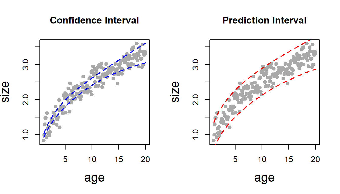
par(mfrow =c(1,2))plot(age, size, pch =19, col ="darkgrey", cex.lab =1.5,main ="Confidence Interval")lines(age, fitted.values(fit)+1.96*sqrt(size_var), col ="blue", lwd =2,lty =2)lines(age, fitted.values(fit)-1.96*sqrt(size_var), col ="blue", lwd =2,lty =2)plot(age, size, pch =19, col ="darkgrey", cex.lab =1.5,main ="Prediction Interval")for(i in1:length(age)){ size_var[i] = (psi_a[i])^2*vcov(fit)[1,1] + (psi_b[i])^2*vcov(fit)[2,2] +2*psi_a[i]*psi_b[i]*vcov(fit)[1,2]+var(residuals(fit))}lines(age, fitted.values(fit)+1.96*sqrt(size_var), col ="red", lwd =2,lty =2)lines(age, fitted.values(fit)-1.96*sqrt(size_var), col ="red", lwd =2,lty =2)
The demonstration of the confidence interval and prediction interval in the context of nonlinear regression model. It can be observed that the prediction interval is wider than the confidence interval. The prediction interval takes the variance of the error component also in account, where the confidence interval considers only the uncertainty associated with the estimated parameters.
12.9 Taylor’s approximation for one variable
In computing the confidence and prediction interval, we have chosen the normal distribution. It is important to check how accurate these approximations are. To understand this concept, we consider a simple example. Suppose that \(X_1,X_2,\ldots,X_n\) be a random sample from the Exponential distribution with rate parameter \(\lambda\). We are interested to estimate the parameter \(\lambda\). We know the following from the Central Limit Theorem that for large \(n\)\[\overline{X_n}\overset{a}{\sim} \mathcal{N}\left(\frac{1}{\lambda}, \frac{1}{\lambda^2 n}\right). \] By the method of moment, we see that the Method of Moment Estimator for \(\lambda\) is \(\frac{1}{\overline{X_n}} = \overline{X_n}^{-1}=\psi\left(\overline{X_n}\right)\) (say).
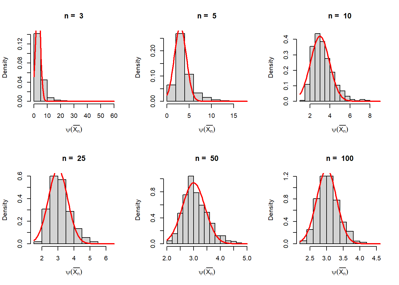
By the first order Taylor’s approximation of \(\psi\left(\overline{X_n}\right)\) about \(\frac{1}{\lambda}\), we obtain \[\psi\left(\overline{X_n}\right) \approx \psi\left(\frac{1}{\lambda}\right) + \left(\overline{X_n}-\frac{1}{\lambda}\right)\psi'\left(\frac{1}{\lambda}\right)\] Now taking expectation on both sides \[\mbox{E}\left[\psi\left(\overline{X_n}\right)\right]\approx \psi\left(\frac{1}{\lambda}\right)=\lambda.\] For computing the variance, we see that \[\mbox{E}\left[\psi\left(\overline{X_n}\right)-\lambda\right]^2\approx \mbox{E}\left[\left(\overline{X_n}-\frac{1}{\lambda}\right)\psi'\left(\frac{1}{\lambda}\right)\right]^2=Var_{\lambda}\left(\overline{X_n}\right)\lambda^4=\frac{\lambda^2}{n},\] provided \(\psi'\left(\frac{1}{\lambda}\right)\ne 0\). Therefore, the approximately \(Var\left(\frac{1}{\overline{X_n}}\right)\approx \frac{\lambda^2}{n}\). Let us verify the same using computer simulation. In addition, we overlay a normal density function with mean \(\lambda\) and variance \(\frac{\lambda^2}{n}\) on the histograms for different values of \(n\). The histograms are simulated using 1000 replications.
par(mfrow =c(2,3))lambda =3n_vals =c(3,5, 10, 25, 50,100)rep =1000for(n in n_vals){ psi_xbar =numeric(length = rep)for(i in1:rep){ x =rexp(n = n, rate = lambda) psi_xbar[i] =1/mean(x) } psi_xbarvar(psi_xbar) lambda^2/nhist(psi_xbar, probability =TRUE, main =paste("n = ", n),xlab =expression(psi(bar(X[n]))))curve(dnorm(x, mean = lambda, sd =sqrt(lambda^2/n)),add =TRUE, col ="red", lwd =2)}
Figure 12.8: As the sample size increases, the sampling distribution of the function of the sample mean is well approximated by a normal distribution. This approximation is known as the Delta method. The histograms are obtained by repeatedly sampling 1000 times from the exponential distribution with rate parameter \(\lambda =3\).
12.10 Bootstrapping regression model
In the following code, we investigate how we can compute the standard of the estimate using the nonparametric bootstrap procedure.
a =1b =0.4age =seq(1, 20, by =0.1)set.seed(123)size = a*age^b +rnorm(n =length(age), mean =0, sd =0.2)plot(age, size, pch =19, col ="darkgrey", cex.lab =1.5)data =data.frame(age, size)B =1000# number of bootstrap data seta_hat =numeric(length = B)b_hat =numeric(length = B)for (i in1:B) { ind =sample(1:nrow(data), replace =TRUE) boot_data = data[ind, ] boot_fit =nls(size ~ a*age^b,data = boot_data,start =list(a =1, b =1)) a_hat[i] =coefficients(boot_fit)[1] b_hat[i] =coefficients(boot_fit)[2]}mean(a_hat) # bootstrap mean
[1] 1.008809
sd(a_hat) # bootstrap standard error or a_hat
[1] 0.02566318
mean(b_hat)
[1] 0.3965658
sd(b_hat)
[1] 0.01025991
Figure 12.9: We fixed the set.seed(123) and simulate the data sets from the population nonlinear regression model. The parameters are fixed as \(a=1\) and \(b=0.4\) and the errors are assumed to be normally distributed. This data set will be resampled to obtain the bootrstrap estimate of the parmaeters and also compute the bootstrap standard error of the estimates.
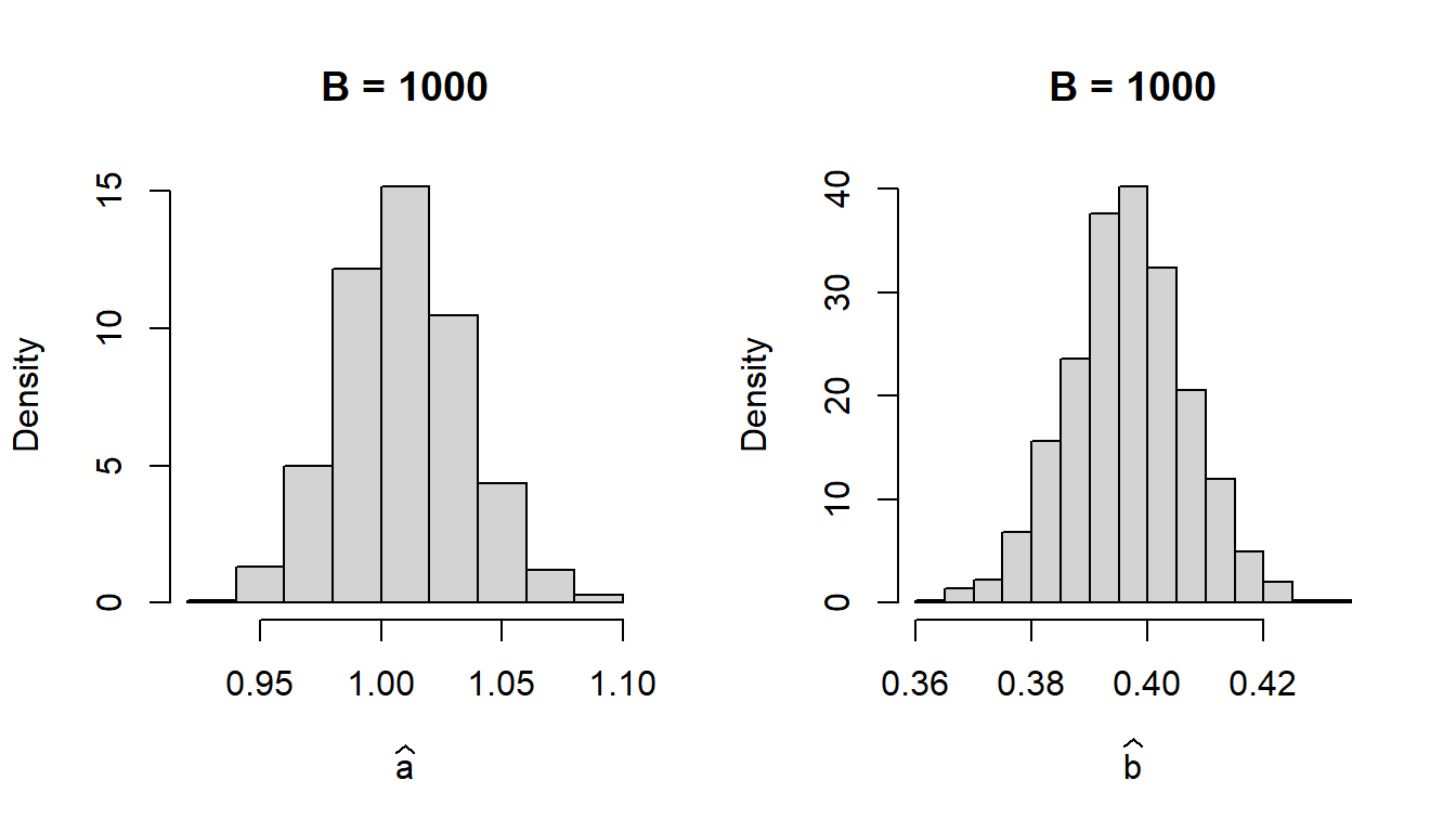
We now visualize the sampling distribution of \(\widehat{a}\) and \(\widehat{b}\) based on \(B=1000\) bootstrap samples.
par(mfrow =c(1,2))hist(a_hat, probability =TRUE,main ="B = 1000", xlab =expression(widehat(a)))cat("95% bootstrap CI for a based on normal distribution is given as \n")
95% bootstrap CI for a based on normal distribution is given as
Figure 12.10: The bootstrap sampling distribution of \(\widehat{a}\) and \(\widehat{b}\) based on 1000 bootstrap samples. It may be noted that the bootstarp estimates are centered about the nls estimates of the parmaeters \(a\) and \(b\) based on the complete data sets, not centered around the true values of \(a\) and \(b\) using which the data has been simulated.
12.11 Case study using synthetic data generation
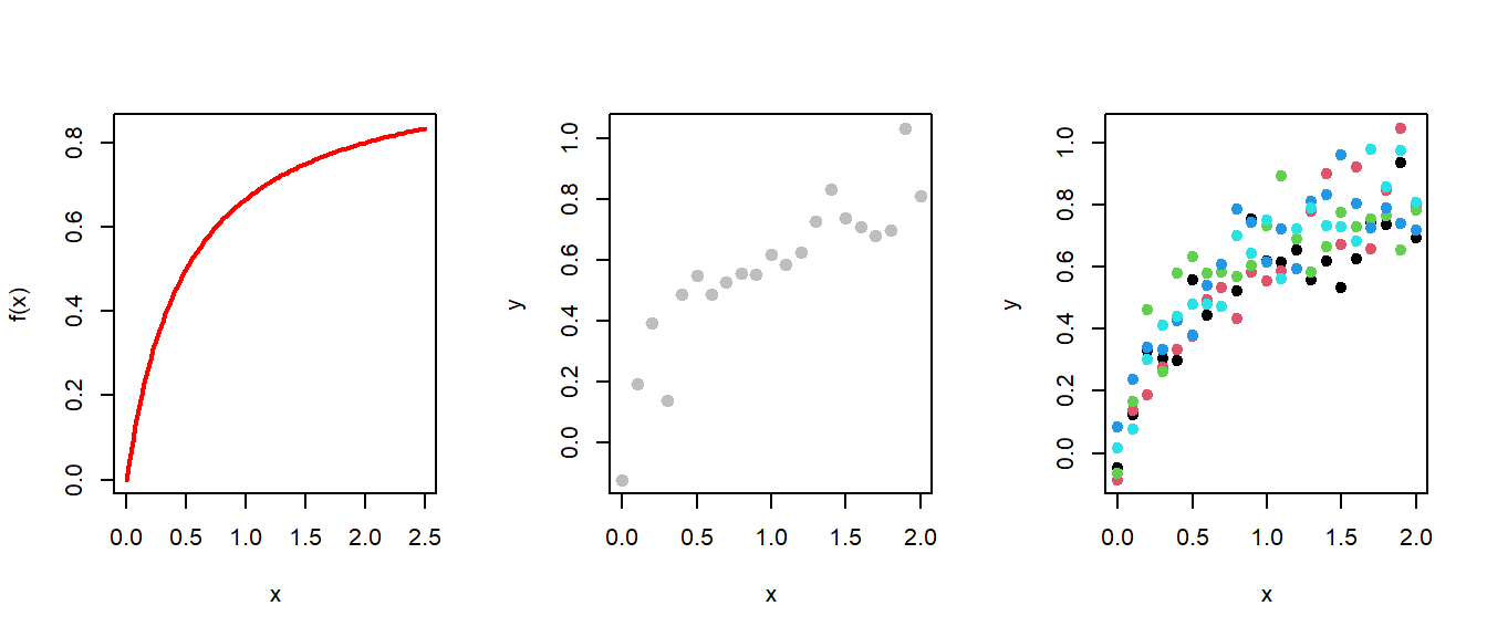
Suppose that we have the population regression function \(f(x|\mathbf{b})\) parameterized by \(\mathbf{b}=(b_0,b_1)'\) and the statistical model for the data is given by \[y_i = f(x|\mathbf{b}) + \epsilon_i = \frac{b_0x}{b_1 + x} + \epsilon_i, i\in \{1,2,\ldots,n\}.\] We assume that the errors \(\epsilon_i\)s are normally distributed with mean \(0\) and variance \(\sigma^2\) and they are also independent. Statisticians formally call it as IID (Independent and Identically Distributed). In following code, we first simulate the synthetic data by fixing the population parameters \(b_0, b_1,\sigma^2\).
par(mfrow =c(1,3))# Plot the mean functionset.seed(1234)b0 =1b1 =0.5f =function(x){ b0*x/(b1+x)}curve(f(x), col ="red", 0, 2.5, lwd =2)sigma2 =0.01# variancex =seq(0, 2, by =0.1)print(x)
plot(x, y, col ="grey", pch =19, cex =1.2)data =matrix(data =NA, nrow =5, ncol =length(x))for(i in1:nrow(data)){ data[i,] = b0*x/(b1+x) +rnorm(n = n, mean =0, sd =sqrt(sigma2))}matplot(x, t(data), col =1:10, pch =19, ylab ="y")
Figure 12.11: The left most panel is the mean population regression function and the right panel contains the simulated data using the seed value 1234. The seed value is used ensure the reproducibility of the plots. For simulation, the parameter choices are set as \(b_0 = 1, b_1 = 0.5, \sigma^2 = 0.01\). In the right most panel some more simulation has been carried to demonstrate the randomness across different simulated data sets.
We consider the minimization of the error sum of squares as the first approach to estimate the parameters. We minimize the following function with respect to \(b_0\) and \(b_1\).
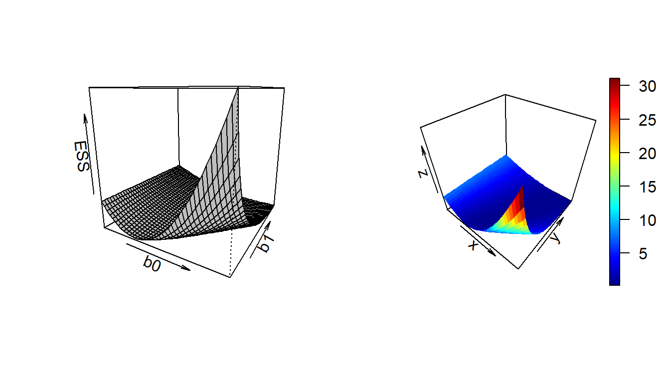
\[\mbox{ESS}(\mathbf{b}) = \sum_{i=1}^n\left(y_i - \frac{b_0 x_i}{b_1+x_i}\right)^2.\] We first plot the surface of the \(\mbox{ESS}(\mathbf{b})\) with different choices of \(b_0\) and \(b_1\). For the user, show the plots using the persp() function and also by using plot3D package.
     [,1] [,2] [,3] [,4] [,5] [,6] [,7] [,8] [,9] [,10] [,11] [,12] [,13] [,14]
[1,]   NA   NA   NA   NA   NA   NA   NA   NA   NA    NA    NA    NA    NA    NA
[2,]   NA   NA   NA   NA   NA   NA   NA   NA   NA    NA    NA    NA    NA    NA
[3,]   NA   NA   NA   NA   NA   NA   NA   NA   NA    NA    NA    NA    NA    NA
[4,]   NA   NA   NA   NA   NA   NA   NA   NA   NA    NA    NA    NA    NA    NA
[5,]   NA   NA   NA   NA   NA   NA   NA   NA   NA    NA    NA    NA    NA    NA
[6,]   NA   NA   NA   NA   NA   NA   NA   NA   NA    NA    NA    NA    NA    NA
     [,15] [,16] [,17] [,18] [,19] [,20] [,21] [,22] [,23] [,24] [,25] [,26]
[1,]    NA    NA    NA    NA    NA    NA    NA    NA    NA    NA    NA    NA
[2,]    NA    NA    NA    NA    NA    NA    NA    NA    NA    NA    NA    NA
[3,]    NA    NA    NA    NA    NA    NA    NA    NA    NA    NA    NA    NA
[4,]    NA    NA    NA    NA    NA    NA    NA    NA    NA    NA    NA    NA
[5,]    NA    NA    NA    NA    NA    NA    NA    NA    NA    NA    NA    NA
[6,]    NA    NA    NA    NA    NA    NA    NA    NA    NA    NA    NA    NA
     [,27] [,28] [,29] [,30] [,31] [,32] [,33] [,34] [,35] [,36] [,37] [,38]
[1,]    NA    NA    NA    NA    NA    NA    NA    NA    NA    NA    NA    NA
[2,]    NA    NA    NA    NA    NA    NA    NA    NA    NA    NA    NA    NA
[3,]    NA    NA    NA    NA    NA    NA    NA    NA    NA    NA    NA    NA
[4,]    NA    NA    NA    NA    NA    NA    NA    NA    NA    NA    NA    NA
[5,]    NA    NA    NA    NA    NA    NA    NA    NA    NA    NA    NA    NA
[6,]    NA    NA    NA    NA    NA    NA    NA    NA    NA    NA    NA    NA
     [,39] [,40]
[1,]    NA    NA
[2,]    NA    NA
[3,]    NA    NA
[4,]    NA    NA
[5,]    NA    NA
[6,]    NA    NA
The left panel shows the surface plto using the persp function and the right panel shows the surface with color gradient.
In the following code, we use the function optim() to minimize the error sum squares function with respect to \(b_0\) and \(b_1\).
out =optim(c(1.5, 1), fn = fun_ESS) # minimize the functionsummary(out)
            Length Class  Mode
par         2      -none- numeric
value       1      -none- numeric
counts      2      -none- numeric
convergence 1      -none- numeric
message     0      -none- NULL
b_hat = out$par # extract the estimatesprint(b_hat)
[1] 1.0820661 0.6865781
In the following, we obtain the estimates of the parameter by using the method of maximum likelihood. The likelihood function is given by
\[\mathcal{L}(\theta) = \prod_{i=1}^n f(y_i|x_i,b_0,b_1,\sigma^2) = \prod_{i=1}^n \frac{1}{\sigma \sqrt{2\pi}}e^{-\frac{1}{2\sigma^2}\left(y_i - \frac{b_0x_i}{b_1+x_i}\right)^2}\] which simplifies to \[\mathcal{L}(b_0,b_1,\sigma^2) = \left(\frac{1}{\sigma^2 2\pi}\right)^{n/2}e^{-\frac{1}{2\sigma^2}\sum_{i=1}^n\left(y_i -\frac{b_0x_i}{b_1 + x_i}\right)^2}.\]
We write down the log-likelihood function as \[l\left(b_0,b_1,\sigma^2\right) = -\frac{n}{2}\log(\sigma^2) - \frac{n}{2}\log(2\pi) - \sum_{i=1}^n\left(y_i -\frac{b_0x_i}{b_1 + x_i}\right)^2.\] Instead of maximizing the log-likelihood function, we can minimize the negative log-likelihood function \(-l(b_0,b_1,\sigma^2)\).
The estimate that we have obtained by employing the method of maximum likelihood is subject to uncertainty due to the random nature of the data set. Therefore, we need to report the uncertainty or the standard error of the estimate. We omit the following result without proof which states that for large sample size the variance covariance matrix of \(\widehat{b_0}\), \(\widehat{b_1}\) and \(\widehat{\sigma^2}\) is well approximated by the inverse of the Hessian matrix evaluated at the MLE with a negative sign.
\[-H = -\begin{bmatrix} \frac{\partial^2 l}{\partial b_0^2} & \frac{\partial^2 l}{\partial b_0 \partial b_1} & \frac{\partial^2 l}{\partial b_0 \partial \sigma^2} \\ \frac{\partial^2 l}{\partial b_0 \partial b_1} & \frac{\partial^2 l}{\partial b_1^2} & \frac{\partial^2 l}{\partial b_1 \partial \sigma^2}\\ \frac{\partial^2 l}{\partial \sigma^2 \partial b_0} & \frac{\partial^2 l}{\partial \sigma^2 \partial b_1} & \frac{\partial^2 l}{\partial (\sigma^2)^2}
\end{bmatrix}_{|_{\left(\widehat{b_0},\widehat{b_1},\widehat{\sigma^2}\right)}}\] In the optim function, we can use the argument \(\texttt{hessian = TRUE}\) to obtain the estimated Hessian matrix at the MLE. In the
out =optim(par =c(1,1,0.1), fn = fun_neglogLik, hessian =TRUE)out$par
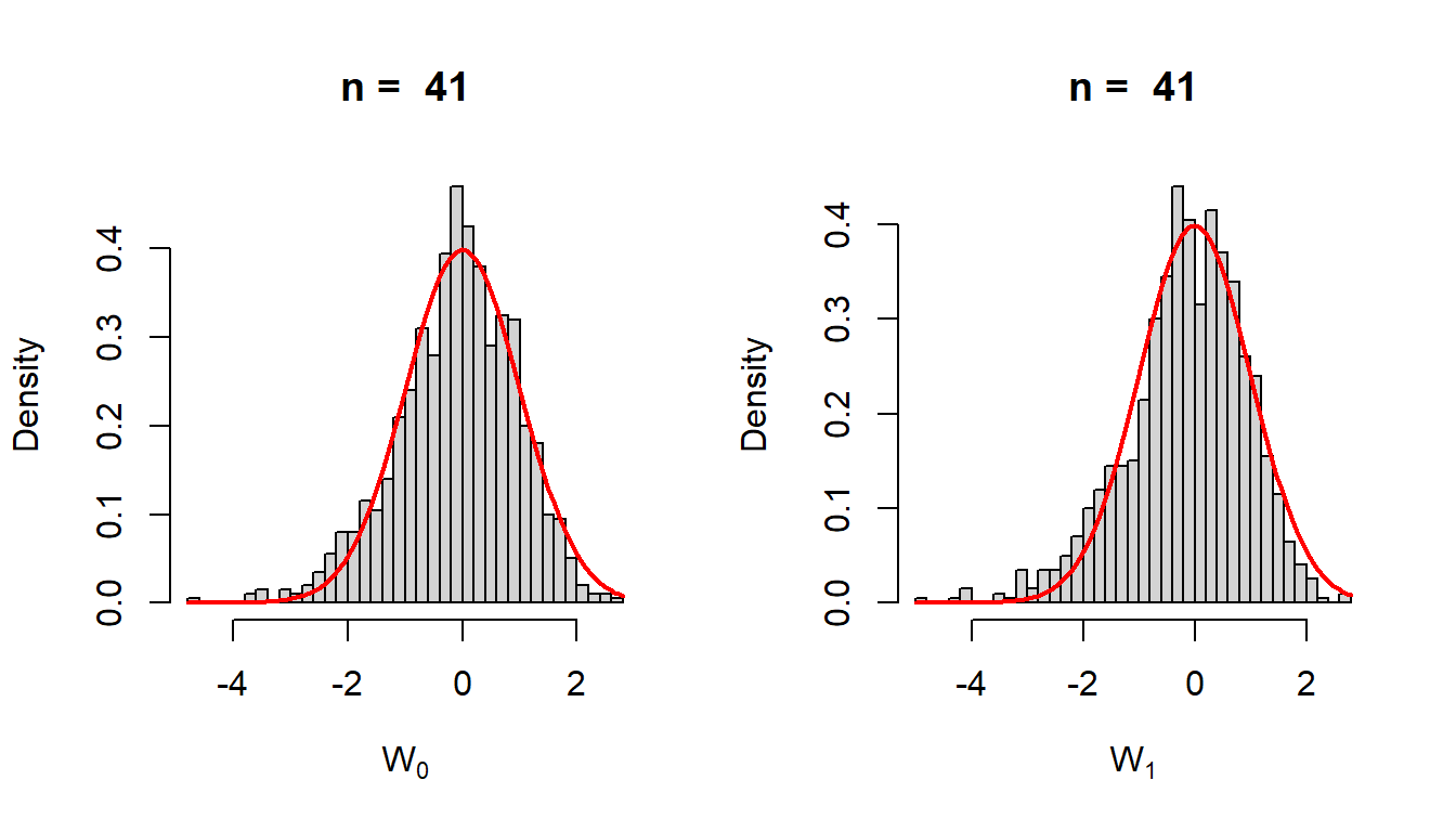
Therefore, the square root of the diagonal entries of the matrix \((-H)^{-1}\) will give the standard error of the MLE. A natural question arises how good these approximations are? To see this, we can visualize the sampling distribution of \[W_0 = \frac{\widehat{b_0}-b_0}{\widehat{\mbox{SE}}(\widehat{b_0})}\] and \[W_1 = \frac{\widehat{b_1}-b_1}{\widehat{\mbox{SE}}(\widehat{b_1})}\] by computer simulation based on 1000 replications.
rep =1000w_0 = w_1 =numeric(length = rep)for(i in1:rep){ x =seq(0, 2, by =0.05) n =length(x) # length of the data y = b0*x/(b1+x) +rnorm(n = n, mean =0, sd =sqrt(sigma2)) out =optim(par =c(1,1,0.1), fn = fun_neglogLik, hessian =TRUE) H = out$hessian w_0[i] = (out$par[1] - b0)/sqrt(solve(out$hessian)[1,1]) w_1[i] = (out$par[2] - b1)/sqrt(solve(out$hessian)[2,2])}par(mfrow =c(1,2))hist(w_0, probability =TRUE, xlab =expression(W[0]),main =paste("n = ", n), breaks =30)curve(dnorm(x), add =TRUE, col ="red", lwd =2)hist(w_1, probability =TRUE, xlab =expression(W[1]),main =paste("n = ", n), breaks =30)curve(dnorm(x), add =TRUE, col ="red", lwd =2)
Figure 12.12: The sampling distribution of the estimator centered at the true value and scaled by the estimated standard error. An approximation with the standard normal distribution is shown for reference.
The simulations suggest that for large sample size \(n\), \[W_0 = \frac{\widehat{b_0} -b_0}{\widehat{\mbox{SE}}(\widehat{b_0})} \sim \mathcal{N}(0,1),\] there for \[\widehat{b_0} \sim \mathcal{N}\left(b_0, \widehat{\mbox{SE}}\left(\widehat{b_0}\right)^2\right),\] for large sample size \(n\). Therefore, large \(n\), \((1-\alpha)\%\) confidence interval for \(b_0\) can be obtained as \[\left(\widehat{b_0} - z_{\alpha/2}\widehat{\mbox{SE}}(\widehat{b_0}), \widehat{b_0} + z_{\alpha/2}\widehat{\mbox{SE}}(\widehat{b_0})\right),\] where \(\mbox{P}(Z>z_{\alpha/2})=\frac{\alpha}{2}\) and \(Z\sim \mathcal{N}(0,1)\).
Classroom Quiz: Simulation
Perform the simulation study with the regression function \[f(x) = \frac{b_0x^2}{b_1^2 + x^2},\] where \(b_0,b_1>0\) and study the sampling distributions of the MLEs.
12.12 Case Study: Local maximization
In the classroom, I have randomly asked Shailaja to suggest a nonlinear function which will be used as the systematic component of the nonlinear regression model to simulate the data. She suggested the following function \[f(x) = \sin(ax) + bx^2, x\in [0,2],\] Therefore, the statistical modelling framework is given by \[y_i = f(x_i) + \epsilon_i,~~i\in\{1,2,\ldots,n\}\] where \(\epsilon_i\sim \mathcal{N}(0,\sigma^2)\). We simulate the data from the above regression model and estimate the model parameters \(a, b, \sigma^2\) using the method of maximum likelihood.
In the first step, we simulate a sample of size \(n\) by fixing the parameters \(a=3, b=1\) and \(\sigma^2 = 0.05\). We use \(\theta = (a,b,\sigma^2)'\) to denote the parameter vector.
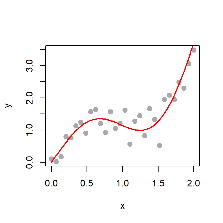
# The mean regression functiona =3b =1f =function(x){sin(a*x) + b*x^2# population nonlinear regression function}n =30# sample sizesigma2 =0.1# population standard deviationx =seq(0, 2, length.out = n) # sequence of x valuesy =numeric(length = n) # for(i in1:n){ y[i] =rnorm(n =1, mean =f(x[i]), sd =sqrt(sigma2))}print(y)
plot(x,y, col ="darkgrey", pch =19, cex =1.2)curve(f(x), add =TRUE, col ="red", lwd =2)
Figure 12.13: The simulated data set and the population regression mean function is overlaid for reference.
In the following R codes, we minimize the negative of the log-likelihood function. The reader is encouraged to write down the expression of the likelihood function explicitly and plot the surface of the likelihood function for different choices of \(a\) and \(b\).
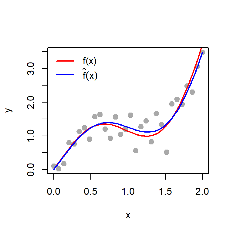
The maximum likelihood estimates of the parameters are given below. In addition, we add both the population nonlinear regression function and the estimated (sample) nonlinear regression function for reference. The estimated regression function is given by \[\widehat{f}(x) = \sin(\widehat{a}x)+\widehat{b}x^2.\]
Figure 12.14: The estimated regression function and the population regression function is shown using different colour and they are in good agreement.
Certainly, the above estimates are subject to uncertainty. Basically, if we simulate another set of data set and compute the MLE, certainly, these estimates are going to differ. However, we want to get an idea, how much they can differ! To obtain the Hessian matrix (\(H\)) will be useful. The estimate of the variance of the MLE of \(\widehat{a}\) is given by \(H^{-1}_{11}\), evaluated at \(\widehat{\theta}\).
To understand the uncertainty associated with these estimates, first we simulate the sampling distribution of \(\widehat{\theta}\) by repeating the simulation experiment \(M\) times. We simulate the sampling distribution of \(\widehat{a}\), \(\widehat{b}\) and \(\widehat{\sigma^2}\).
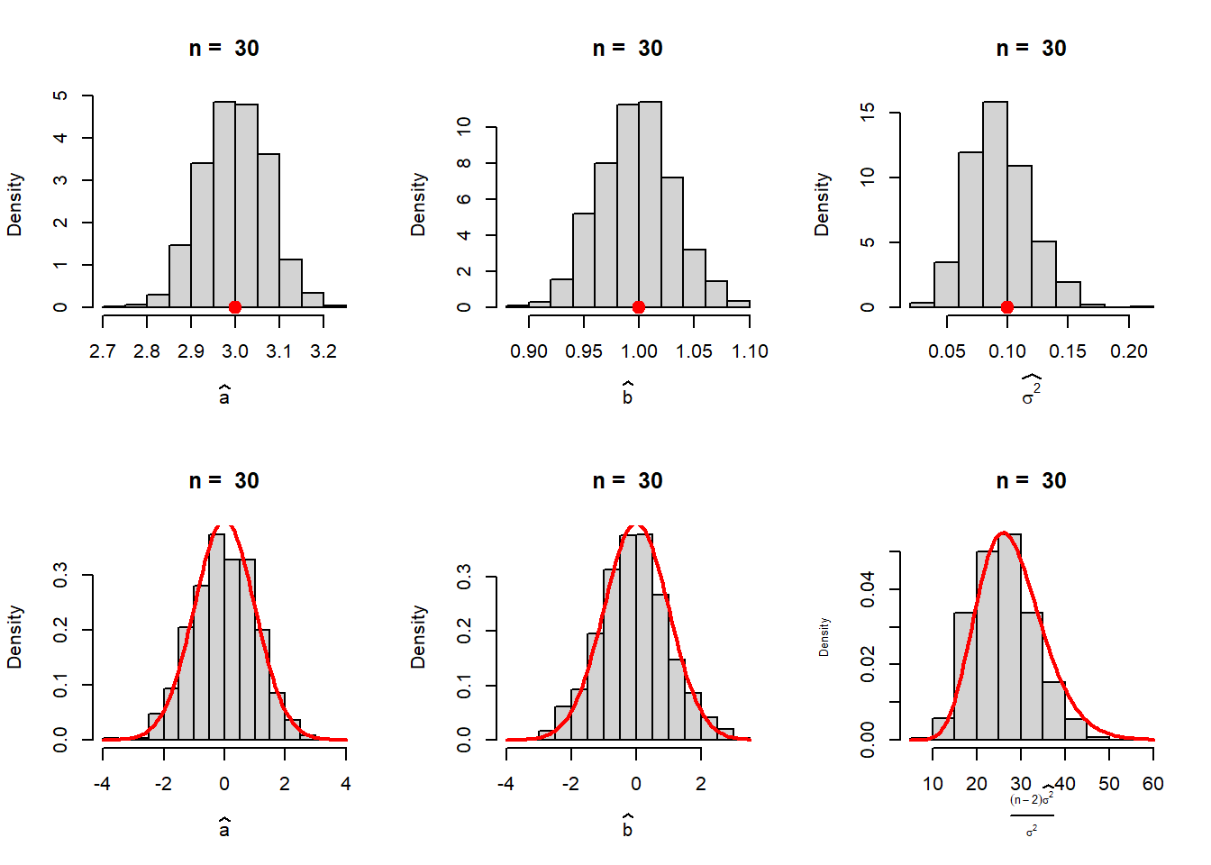
We also compute the following three quantities: \[W_a = \frac{\widehat{a} - a}{\widehat{\mbox{SE}}(\widehat{a})},~~~~~~W_b = \frac{\widehat{b} - b}{\widehat{\mbox{SE}}(\widehat{b})},~~~~W_{\sigma^2} = \frac{(n-2)\widehat{\sigma^2}}{\sigma^2}.\]
M =1000a_hat =numeric(length = M)b_hat =numeric(length = M)sigma2_hat =numeric(length = M)se_a_hat =numeric(length = M)se_b_hat =numeric(length = M)se_sigma2_hat =numeric(length = M)for (j in1:M) { x =seq(0, 2, length.out = n) y =numeric(length = n)for(i in1:n){ y[i] =rnorm(n =1, mean =f(x[i]), sd =sqrt(sigma2)) } out =optim(par =c(2.8,0.9,0.04), fn = fun_neglogLik,hessian =TRUE) a_hat[j] = out$par[1] b_hat[j] = out$par[2] sigma2_hat[j] = out$par[3] H = out$hessian se_a_hat[j] =sqrt(solve(H)[1,1]) se_b_hat[j] =sqrt(solve(H)[2,2]) se_sigma2_hat[j] =sqrt(solve(H)[3,3])}par(mfrow =c(2,3))hist(a_hat, probability =TRUE, xlab =expression(widehat(a)),main =paste("n = ", n))points(a, 0, pch =19, cex =1.5, col ="red")hist(b_hat, probability =TRUE, xlab =expression(widehat(b)),main =paste("n = ", n))points(b, 0, pch =19, cex =1.5, col ="red")hist(sigma2_hat, probability =TRUE, xlab =expression(widehat(sigma^2)),main =paste("n = ", n))points(sigma2, 0, pch =19, cex =1.5, col ="red")hist((a_hat-a)/se_a_hat, probability =TRUE, xlab =expression(widehat(a)),main =paste("n = ", n))curve(dnorm(x), add =TRUE, col ="red", lwd =2)hist((b_hat-b)/se_b_hat, probability =TRUE, xlab =expression(widehat(b)),main =paste("n = ", n))curve(dnorm(x), add =TRUE, col ="red", lwd =2)hist((n-2)*sigma2_hat/sigma2 , probability =TRUE, xlab =expression(over((n-2)*widehat(sigma^2),sigma^2)),main =paste("n = ", n), cex.lab =0.6)curve(dchisq(x, df = n-2), add =TRUE, col ="red", lwd =2)
Figure 12.15: The top panel represents the simulated sampling distribution of the MLEs based on \(M=1000\) replications. The over red dot indicates the true value of the parameters using which the training data sets have been simulated. It is interesting to see that, MLEs are centered about the true valye, ensuring unbiasedness of the MLE. In the lower panel, the simulated distributions of \(W_a\), \(W_b\) and \(W_{\sigma^2}\) are drawn. The standard normal distribution is overlaid on the first two histograms (bottom panel) and the last figure is overlaid with a \(\chi^2\) distribution with \((n-2)\) degrees of freedom.
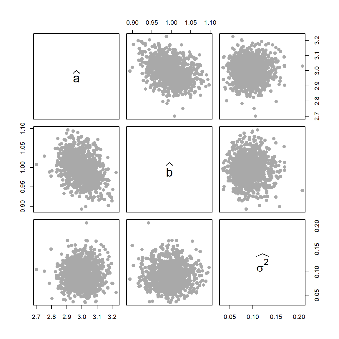
pairs(theta_hat, col ="darkgrey", pch =19, cex =1.2,labels =c(expression(widehat(a)), expression(widehat(b)), expression(widehat(sigma^2))))
Figure 12.16: The pairs plot indicates a small negative correlations between \(\widehat{a}\) and \(\widehat{b}\), whereas, these estimators are independent with \(\widehat{\sigma^2}\)
12.12.1 Sensitivity to the Initial Conditions
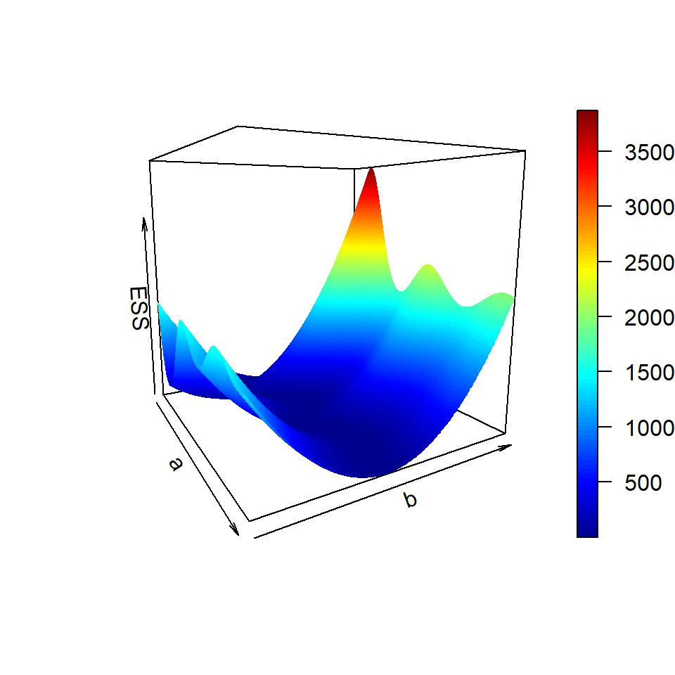
In the following, we visualize the error sum of squares as a function \(a\) and \(b\). The surface clearly demonstrates the existence of multiple local minimum and depending upon the initial conditions different minimum will be achieved.
Figure 12.17: The surface of the negative log likelihood function for a specific choice of \(\sigma^2\). Here we plot the error sum of squares, however, one must note that under the normality assumption, the surface is proportional to the negative log-likelihood function.