We start our discussion of today’s lecture with the usual multiple linear regression using the matrix set up which is given by \[Y_{n\times 1} = X_{n\times (p+1)}\beta_{(p+1)\times 1} + \epsilon_{n\times 1},\] and the symbols have the standard interpretations.
In addition, we assume that \(\epsilon_{n\times 1} \sim \mathcal{N}_n\left(0_{n\times 1}, \sigma^2I_{n\times n}\right)\). We have also checked in the class that \(\mbox{E}(\widehat{\beta}) =\beta\) that means the estimator \(\widehat{\beta}\) an unbiased estimator of \(\beta\). To recall that \[\widehat{\beta} = \mbox{argmax}_{\beta}(Y-X\beta)'(Y-X\beta).\]
The covariance matrix of \(\widehat{\beta}\) is given by \[Cov(\beta) = \sigma^2(X'X)^{-1}.\] The diagonal entries of the above matrix gives us the variance associated with the estimator for individual component \(\beta_j\) of \(\beta\) for \(j\in \{0,1,2,\ldots,p\}\). It is important to note that if the matrix \((X'X)\) is nearly singular, or ill conditioned, then the determinant \(|X'X|\approx 0\) and the variance \(Var(\widehat{\beta_j})\) for \(j\in\{0,1,\ldots,p\}\) will be large and the estimates will unreliable. By unreliable, I mean the standard error of the estimators will be extremely large or may be infinity as well.
A natural question arises, in what scenarios such a possibility arise. From the theory of linear algebra, we know that if one column can be written as a constant multiple of another column, the determinant of the matrix is zero. It is not only between two columns, if a column can be written as a linear combination of two or more other columns (with at least one non-zero coefficient), then also the determinant is zero. In other words, the column space of the matrix does not have the dimension equal to the number of columns of \(X\). In other words, the columns are linearly dependent.
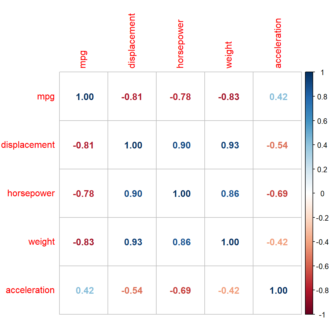
Given the above discussion, if we want to avoid such situation where \(|X'X|\approx 0\), we need to identify which columns of \(X\) are responsible for this. While discussing the concept of correlation, we have emphasized the fact that the correlation is a measure of linear relationship between random variables. Therefore, the degree of linear dependence between two columns of \(X\) (also called feature by machine learning experts) can be measured by the correlation between two columns of \(X\). However, when one column can be written as a linear combination of other columns, that correlation may not be able to capture. Such dependence can be checked by fitting linear regression of the following form \[X_j = \beta_0^{(-j)} + \beta_1^{(-j)}X_1 + \cdots+\beta_{j-1}^{(-j)}X_{j-1}+\beta_{j+1}^{(-j)}X_j + \beta_pX_p + \epsilon\] for \(j\in \{1,2,\ldots,p\}\). A large r.squared value of the above regression model \(R_{-j}^2\) indicates that \(X_j\) can be approximately represented as a linear combination of other columns.
Data scientists computes the quantity called, variance inflation factor (VIF) by \[\mbox{VIF}_j = \frac{1}{1-R_{-j}^2}, j=1,2,\ldots,p.\] If the variance inflation factor is more than 5 or 10 (depending on the problem and also domain knowledge), an analyst may choose to drop those variables.
Let us consider the \(\texttt{Auto}\) dataset from the ISLR2 package in R.
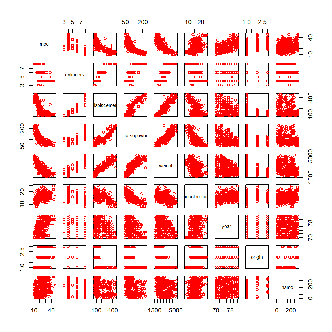
library(ISLR2)pairs(Auto, col ='red')
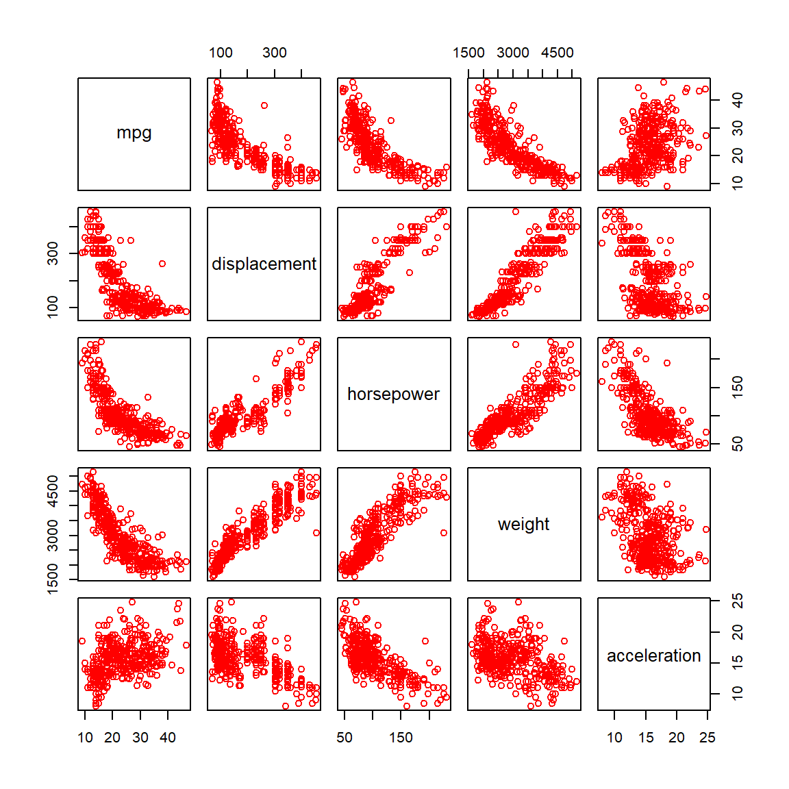
Pairs plot for the Auto data set with five selected columns.
data = Auto[,c("mpg", "displacement", "horsepower", "weight", "acceleration")]head(data)
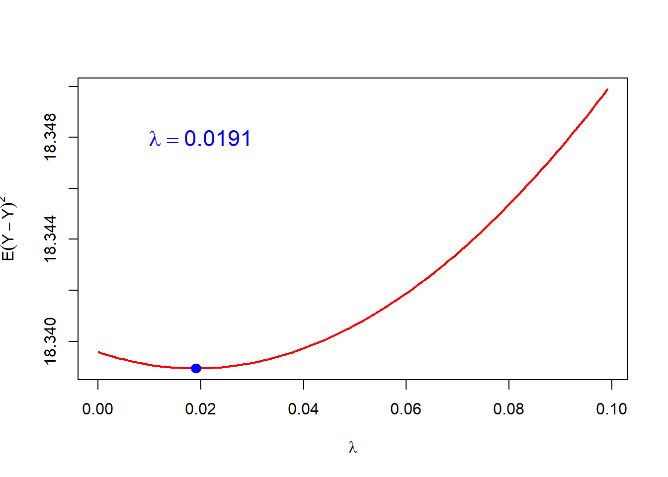
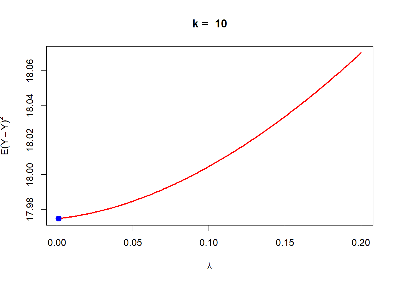
lambda_star = lambda_vals[which.min(pred_error)]points(lambda_star,pred_error[which.min(pred_error)],pch =19, col ="blue",cex =1.3)text(0.02, 18.348, bquote(lambda == .(lambda_star)),cex =1.4, col ="blue", pch =19, bty ="n")
In the above analysis, it is clear that the computation associated with the approximation of the prediction error is heavy. The number of rows in the data set is 392, therefore, 392 many times, model training has been carried out. The advantage of the above method is basically is that every row of the data set has been used for both model training as well as model testing purpose. The number of model fitting exercises may be reduced by dividing the data into \(k\) many segments of approximately equal size.
nrow(data)
[1] 392
Y = data$mpgX =cbind(rep(1,nrow(data)), as.matrix(data[,-1]))Y