mu = 3                        # population mean
sigma = 1                     # population standard deviation
f = function(x){
  dnorm(x, mean = mu, sd = sigma)
}
curve(f(x), col = "red", lwd = 2, -3, 9)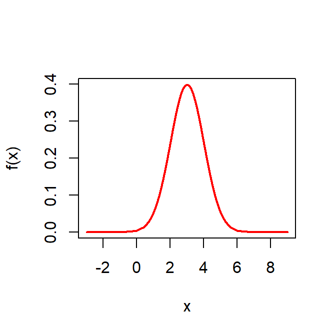
In a typical statistics classroom, the teacher often begins by discussing either a coin-tossing experiment or by collecting data randomly from a normally distributed population, with the goal of estimating the probability of success or the population mean, respectively. In both cases, no actual statistical sampling occurs; instead, students are asked to imagine a hypothetical experiment carried out by the teacher, calculating the sample proportion or sample mean based on imagined sample data. Consequently, students often miss the actual connection between fixed sample values (obtained once data is collected) and theoretical probability density functions (which are purely mathematical constructs).
This gap in understanding could be greatly reduced if real-time random experiments were conducted in the classroom, similar to experiments in Physics, Chemistry, Biology, or Engineering courses. By utilizing software that can simulate various probability distributions, we can bridge this gap and enhance comprehension. This chapter is developed to facilitate an understanding of randomness in various computations based on sample data using computer simulations. Concepts that are often only intuitively grasped can, through simulated experiments, be transformed into concrete understanding. This document contains several R codes developed during the lectures on Statistical Computing for students enrolled in the Multidisciplinary Minor Degree Programme in Machine Learning and Artificial Intelligence, offered by the Department of Mathematics, Institute of Chemical Technology, Mumbai, under the umbrella of the National Education Policy NEP 2020. I extend my heartfelt thanks to all the students for their excellent support during the lectures and for inspiring me to simulate theoretical concepts for practical illustration.
If we set up a simulation experiment, the first task is to assume the population distribution. In this case, we start our discussion with the normal distribution and we use the symbol \(f(\cdot)\) to represent the population PDF or PMF throughout this chapter. Suppose that we consider problem of estimating the mean of the population distribution \(\mathcal{N}(\mu,\sigma^2)\).
mu = 3 # population mean
sigma = 1 # population standard deviation
f = function(x){
dnorm(x, mean = mu, sd = sigma)
}
curve(f(x), col = "red", lwd = 2, -3, 9)In practice while teaching, the drawing of the histogram of the sampled data has been a very effective way to bridge the connection between the theoretical PDF and the sample.
n = 50                                           # sample size
x = rnorm(n = n, mean = mu, sd = sigma)
print(x)
[1] 1.671086 2.225304 1.529958 2.204676 1.911372 2.560277 3.915540 3.104654
[9] 2.942460 3.491619 2.921612 4.714862 1.790840 3.576951 2.889409 3.831369
[17] 2.346119 1.665619 3.230136 2.345178 3.115959 3.297198 2.516690 1.942996
[25] 4.360242 4.631048 3.998281 4.671506 3.594069 4.156748 4.148623 3.879374
[33] 3.518967 2.652628 1.587910 3.292323 4.050451 2.454345 1.480163 3.128216
[41] 1.600328 2.946126 2.866553 2.525534 4.699478 4.866882 4.127249 2.009809
[49] 3.166133 1.793613hist(x, probability = TRUE)
curve(f(x), add= TRUE, col = "red", lwd = 2)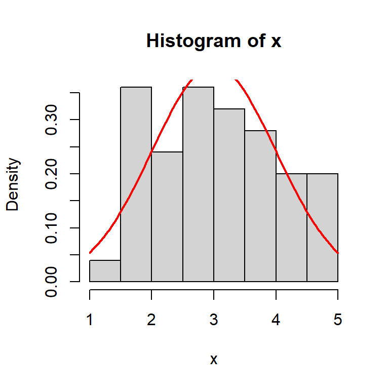
sample_mean = mean(x)
sample_var = var(x)
cat("The sample mean and variance are\n")
The sample mean and variance areprint(sample_mean)[1] 3.03897print(sample_var)[1] 0.9742523Invariably, the sample mean will keep on changing as we execute the step - I and step - II multiple times as different run will give different set of random samples. To understand the sampling distribution of the sample mean, we repeat the above process \(m = 1000\) times and approximate the actual probability density of the sample mean by using histograms.
m = 1000
sample_mean = numeric(length = m)
for(i in 1:m){
  x = rnorm(n = n, mean = mu, sd = sigma)
  sample_mean[i] = mean(x)
}
hist(sample_mean, probability = TRUE, main = paste("n = ",n),
     xlab = expression(bar(X[n])))
points(mu, 0, pch = 19, col = "red", lwd = 2, cex = 1.3)
points(mean(sample_mean), 0, col = "blue", lwd = 2, cex = 1.5)


cat("The average of the 1000 many sample mean values is \n")
The average of the 1000 many sample mean values is print(mean(sample_mean))[1] 2.996231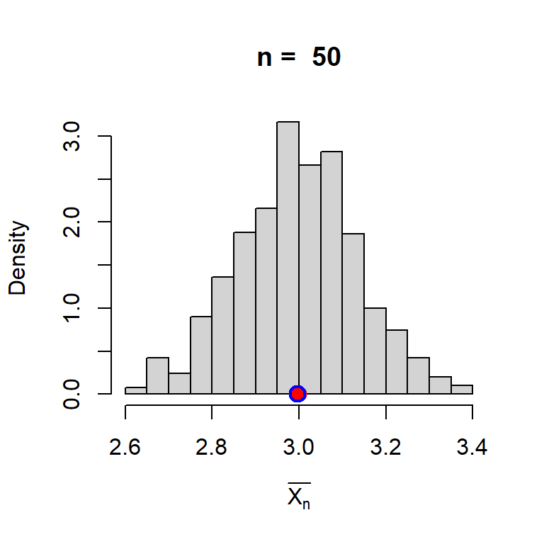
In the above simulation experiment, what are your observations if you perform the following:
Let us do this experiment for different sample sizes and see how the distribution behaves. Our theory suggested that \(\mbox{E}(\overline{X_n}) = \mu\), that is, the sample mean is an unbiased estimator of population mean and the expected value does not depend on \(n\).
par(mfrow = c(1,3))
m = 1000
n_vals = c(3,10,25)
for(n in n_vals){
  sample_mean = numeric(length = m)
  for(i in 1:m){
    x = rnorm(n = n, mean = mu, sd = sigma)
    sample_mean[i] = mean(x)
  }
  hist(sample_mean, probability = TRUE, main = paste("n = ", n),
       xlim = c(1,5))
  points(mu, 0, pch = 19, col = "red", lwd = 2, cex = 1.3)
  points(mean(sample_mean), 0, col = "blue", lwd = 2,
         cex = 1.5)
}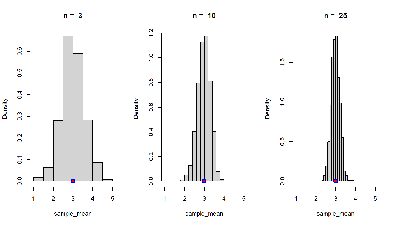
In the simulation (Step - IV), the true population mean is indicated using the red dot and the average of the sample means based on 1000 replication is shown using blue circle. The averaging of the sample mean values can be thought of as an expected value of \(\overline{X_n}\), that is, \(\mbox{E}\left(\overline{X_n}\right)\). This simulation gives an idea that \(\mbox{E}\left(\overline{X_n}\right)\) is equal to the true population mean \(\mu\) (here it is \(1\)). Although not a mathematical proof, but such simulation outcomes gives an indication of the unbiasedness of the sample mean.
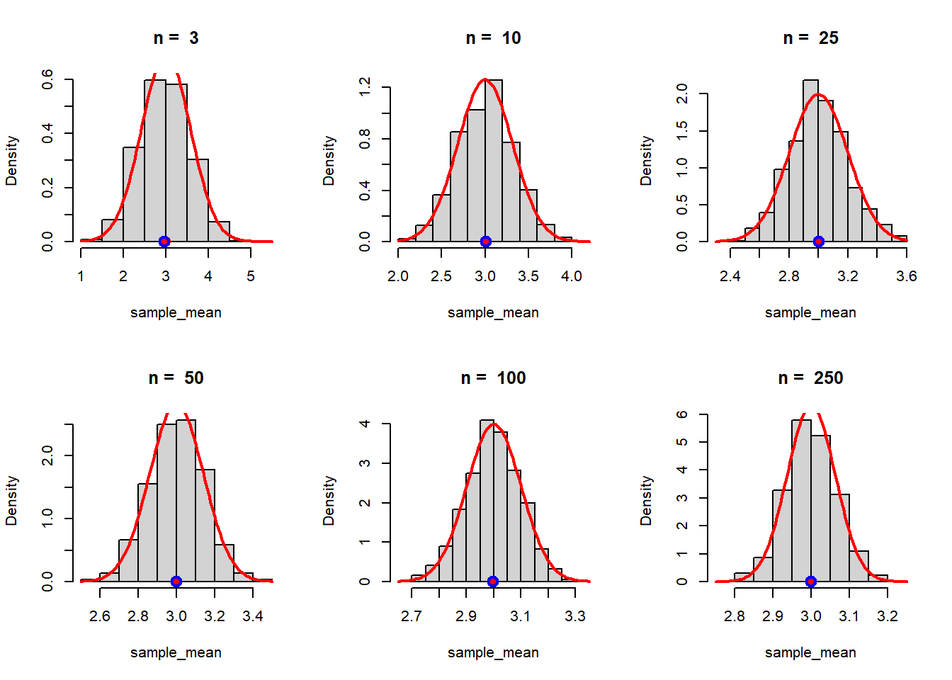
In theory, we have computed by using Moment Generating Functions that \[\overline{X_n} \sim \mathcal{N}\left(\mu, \frac{\sigma^2}{n}\right).\] Let us check whether the theoretical claim can be verified by using simulation.
par(mfrow = c(2,3))
n_vals = c(3, 10, 25, 50, 100, 250)
m = 1000
for(n in n_vals){
  sample_mean = numeric(length = m)
  for(i in 1:m){
    x = rnorm(n = n, mean = mu, sd = sigma)
    sample_mean[i] = mean(x)
  }
  hist(sample_mean, probability = TRUE, main = paste("n = ", n))
  points(mu, 0, pch = 19, col = "red", lwd = 2, cex = 1.3)
  points(mean(sample_mean), 0, col = "blue", lwd = 2,
         cex = 1.5)
  curve(dnorm(x, mean = mu, sd = sqrt(sigma^2/n)),
        add = TRUE, col = "red", lwd = 2)

}
A natural question asked by the students was that how we were actually writing \(\mbox{E}(X_1) = \mu\) and \(Var(X_1) = \sigma^2\). In fact, the question is much deeper which states that what do we really mean by writing \(X_1,X_2,\ldots,X_n\) are independent and identically distributed random variables each having the same population distribution. \[X_1,X_2, \ldots,X_n \sim \mathcal{N}(\mu,\sigma^2)\]
From a simulation perspective, if we want to check whether \(X_1\) follows the same population distribution, we need to repeat the sampling \(m=1000\) times (say) and from each sample of size \(n\), we record the first entry, which is a realization of \(X_1\).
In the following, we do this process for \(n = 3\). Let us write down the steps in algorithmic way:
n = 3
M = 1000
mu = 3; sigma = 1
x1_vals = numeric(length = M)
x2_vals = numeric(length = M)
x3_vals = numeric(length = M)
for(i in 1:M){
  x = rnorm(n = n, mean = mu, sd = sigma)
  x1_vals[i] = x[1]
  x2_vals[i] = x[2]
  x3_vals[i] = x[3]
}
par(mfrow = c(1,3))
hist(x1_vals, probability = TRUE, xlab = expression(X[1]),
     main = paste("n = ", n))
curve(dnorm(x, mean = mu, sd = sigma), add = TRUE,
      col = "red", lwd = 2)
hist(x2_vals, probability = TRUE, xlab = expression(X[2]),
     main = paste("n = ", n))
curve(dnorm(x, mean = mu, sd = sigma), add = TRUE,
      col = "red", lwd = 2)
hist(x3_vals, probability = TRUE, xlab = expression(X[3]),
     main = paste("n = ", n))
curve(dnorm(x, mean = mu, sd = sigma), add = TRUE,
      col = "red", lwd = 2)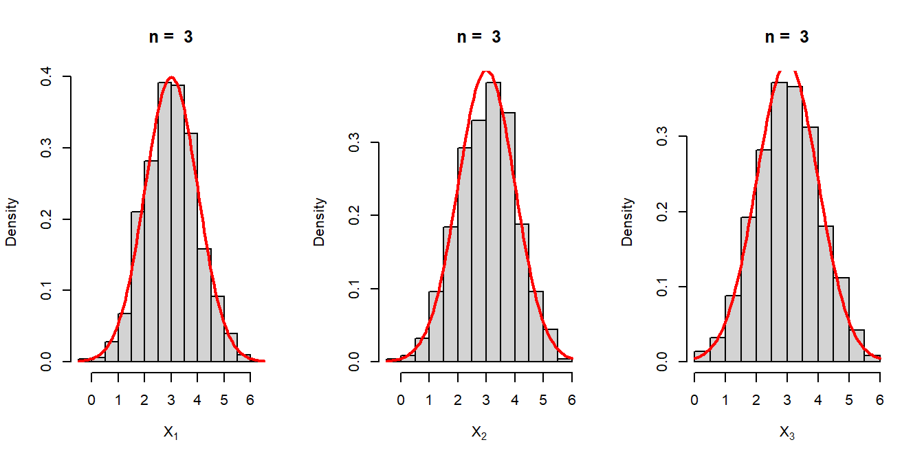
Suppose that \(\{X_n\}\) be a sequence of random variables defined on some probability space \((\mathcal{S}, \mathcal{B},\mbox{P})\) and \(X\) be another random variable defined on the same probability space. We say that the sequence \(\{X_n\}\) converges to \(X\) in probability, denoted as \(X_n \overset{P}{\to} X\), if for any \(\epsilon>0\) (however small), the following condition holds \[\lim_{n\to\infty }\mbox{P}\left(\left|X_n-X\right|\ge \epsilon\right) = 0.\] Basically for every \(X_n\), we construct a sequence of real numbers \((a_n)\) obtained by \[a_n = \mbox{P}\left(\left|X_n-X\right|\ge \epsilon\right)=\int\int_{\{(x_n,x)\colon |x_n-x|\ge \epsilon\}}f_{X_n,X}\left(x_n,x\right)dx_n dx.\] If \(\lim_{n\to\infty}a_n = 0\), then the sequence of random variables \(\{X_n\}\) converges to \(X\) in probability. Let us consider a simple example.
Suppose \(\{X_n\}\) be a sequence of independent random variables having \(\mbox{Uniform}(0,\theta), \theta\in(0,\infty)\) distribution. Consider the following sequence of random variables \[Y_n = \max(X_1,X_2,\ldots,X_n)\] which is also known as the maximum order statistics. We show that \(Y_n\to \theta\) in probability. First of all, we compute the sampling distribution of \(Y_n\). We first find the CDF of \(Y_n\) and by differentiating the CDF, we can obtain the PDF \(f_{Y_n}(y)\).
\[\begin{eqnarray} F_{Y_n}(y) &= \mbox{P}\left(Y_n\le y\right) = \mbox{P}\left(\max(X_1,\ldots,X_n)\le y\right)\\ &= \mbox{P}\left(X_1\le y, X_2\le y,\ldots,X_n\le y\right)\\ &=\mbox{P}\left(X_1\le y\right)\cdots \left(X_n\le y\right)\\ &=\left(\mbox{P}\left(X_1\le y\right)\right)^n = \left(\frac{y}{\theta}\right)^n, 0<y<\theta. \end{eqnarray}\]
By differentiating the CDF, we obtain the PDF as \[f_{Y_n}(y) = n\left(\frac{y}{\theta}\right)^{n-1}\frac{1}{\theta}, 0<y<\theta,\] and zero, otherwise. Before going to the mathematical proof, let us consider the following simulation exercises. In the following we obtain the sampling distribution of \(Y_n\) based on computer simulation using the following algorithm:
In the above step, at each step \(j\in\{1,2,\ldots,m\}\) we fix , so that the figures are reproducible. In the following codes, we do the same experiment for minimum order statistics as well which is given by \[Y_1 = \min(X_1,X_2,\ldots,X_n).\]
theta = 1
n = 10
x = runif(n = n, min = 0, max = theta)
# print(x)
print(max(x))
[1] 0.7960866m = 1000
y_1 = numeric(length = m)
y_n = numeric(length = m)
for(i in 1:m){
set.seed(i)
x = runif(n = n, min = 0, max = theta)
y_1[i] = min(x)
y_n[i] = max(x)
}
par(mfrow = c(1,2))
hist(y_1, probability = TRUE, main = paste("n = ", n),
xlab = expression(Y[1]), breaks = 30)
curve(n*(1-x/theta)^(n-1)*(1/theta), add= TRUE, col = "red",
lwd = 2)
hist(y_n, probability = TRUE, main = paste("n = ", n),
xlab = expression(Y[n]), breaks = 30)
curve(n*(x/theta)^(n-1)*(1/theta),
add = TRUE, col = "red", lwd = 2)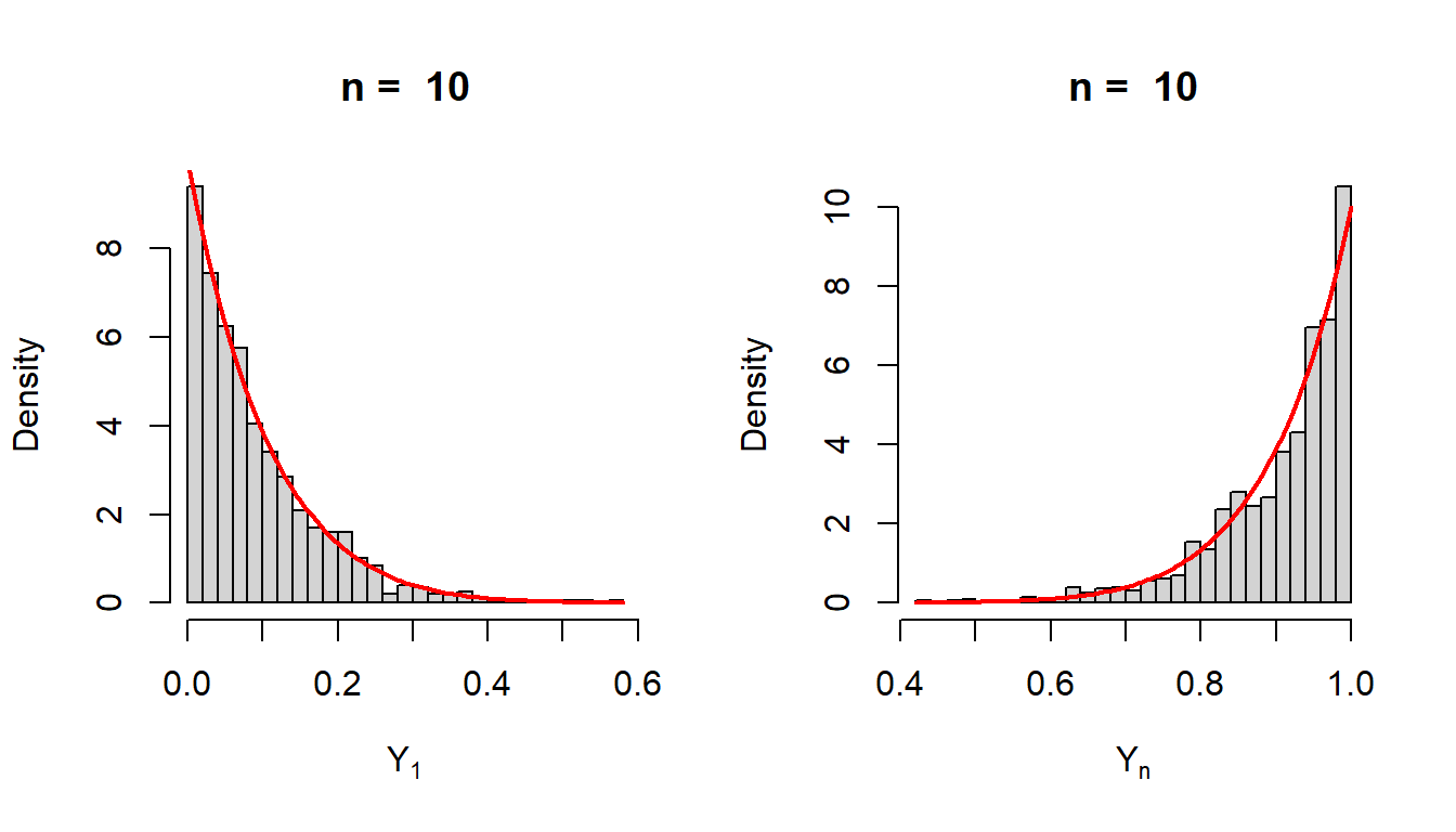
The exact sampling distribution of the minimum order statistics \(Y_1\) can be derived in a similar fashion. First, we compute the CDF of \(Y_1\).
\[\begin{eqnarray} F_{Y_1}(y) &=& \mbox{P}(Y_1\le y)=1- \mbox{P}(Y_1>y)\\ &=&1-\mbox{P}\left(\min(X_1,X_2,\ldots,X_n)>y\right)\\ &=&1-\mbox{P}\left(X_1>y,\ldots,X_n>y\right)\\ &=&1-\prod_{i=1}^n\mbox{P}\left(X_i>y\right)=1-\left(1-\mbox{P}(X_1\le y)\right)^n=1-\left(1-\frac{y}{\theta}\right)^n, 0<y<\theta. \end{eqnarray}\]
The PDF of \(Y_1\) is given by \[f_{Y_1}(y)= \begin{cases}n\left(1-\frac{y}{\theta}\right)^{n-1}\frac{1}{\theta}, ~~0<y<\theta\\ 0,~~~~~~~~~~~~~~ ~~~~~~~~~~~~\mbox{Otherwise}. \end{cases}\]
In the above explanation, we have fixed the sample size \(n\) and simulated the observations from the sampling distribution of \(Y_1\) and \(Y_n\). The process is repeated 1000 times and check whether the resulting histograms are well approximated by the theoretically derived PDFs. In the following, we vary \(n\in\{1,2,3\ldots\}\) and for each \(n\), we simulate a random sample of size \(n\) and compute \(Y_1\) and \(Y_n\). Therefore, in this scheme, we do not have any replications. We plot the sequences \(\{Y_1^{(1)}, Y_1^{(2)},\ldots\}\) and \(\{Y_n^{(1)}, Y_n^{(2)},\ldots\}\) values against \(n\in\{1,2,3\ldots\}\). This will give an idea, as sample size increases, whether these random quantities converge to some particular values.
n_vals = 1:100
y_1 = numeric(length = length(n_vals))
y_n = numeric(length = length(n_vals))
for(n in n_vals){
  x = runif(n = n, min = 0, max = theta)
  y_1[n] = min(x)
  y_n[n] = max(x)
}
plot(n_vals, y_n, type = "p", col = "red", lwd = 2,
     xlab = "sample size (n)", ylim = c(0,1), ylab = " ")
lines(n_vals, y_1, col = "blue", type = "p", lwd = 2)
legend(50, 0.5, legend = c(expression(Y[1]), expression(Y[n])),
       col = c("blue", "red"), bty = "n", lwd =c(2,2))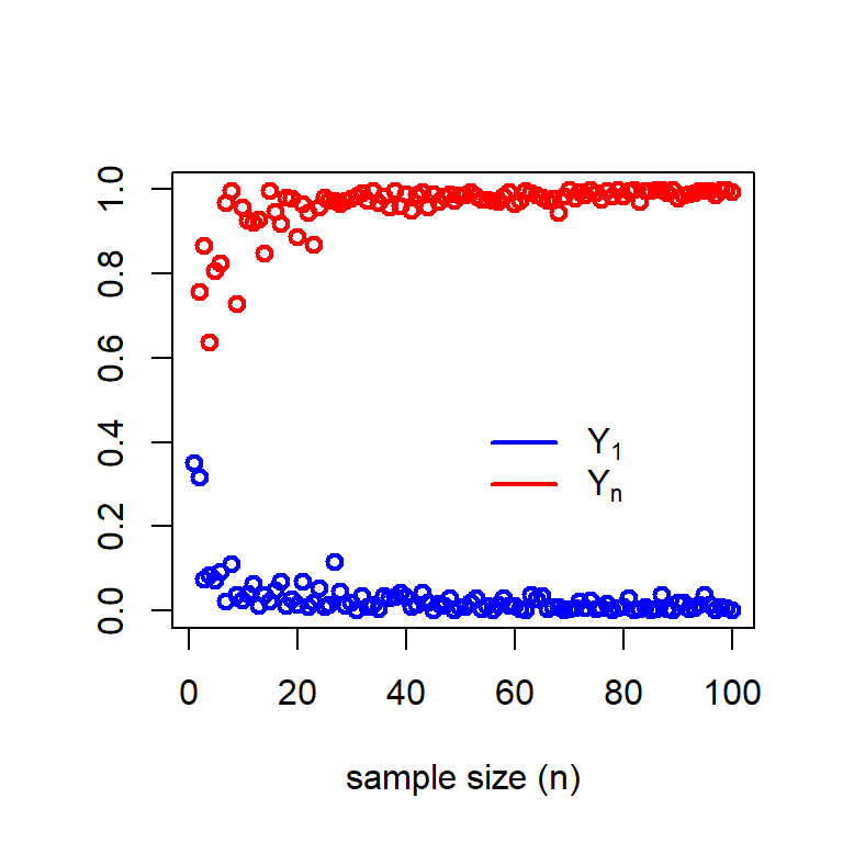
The Central Limit Theorem is one of the most fundamental concepts in Statistics which has profound applications across all domains of Data Science and Machine Learning. It says that the sample mean is approximately normally distributed for large sample size \(n\). However, we shall see it more critically and what are the assumptions needed to understand it in a better way. We shall see some mathematical proof and a lots of simulation to understand this idea better. To understand CLT, first we understand the concept of the convergence in distribution. We elaborate it using a couple of motivating examples along with visualization using R.
Suppose that \(X_1, X_2, \ldots,X_n\) be a sequence of random variables follows \(\mbox{Uniform}(0,\theta)\) distribution, where \(\theta \in(0,\infty) = \Theta\) (say). Suppose that \(Y_n\) be the maximum order statistics whose CDF is given by \[F_n(x) = \mbox{P}(Y_n\le x) = \begin{cases} 0,~~~~~~~ -\infty<x<0,\\ \left(\frac{x}{\theta}\right)^n, 0 \le x<\theta,\\ 1, ~~~~~~~\theta\le x<\infty.\end{cases}\] We are interested to know as \(n\to \infty\), how the function \(F_n(x)\) behaves at each value of \(x\). If is easy to observe that
Therefore, the limiting CDF is given by the following function which represents the CDF of a random variable \(X\) which takes the value \(\theta\) with probability \(1\). \[F_X(x) = \begin{cases} 1, \theta\le x<\infty \\ 0, -\infty <x<\theta.\end{cases}\] In the following, we see visualize the convergence graphically. It is important to note that each \(F_n(x)\) is a continuous function for \(n\in\{1,2,3\ldots\}\), however the limiting CDF is not continuous at \(x=0\). We say that the maximum order statistics \(Y_n = \max(X_1,X_2,\ldots,X_n)\) converges in distribution to the random variable \(X\).
theta = 2
n = 1
F_n = function(x){
  (x/theta)^n*(0<=x)*(x<theta) + (theta<=x)
}
curve(F_n(x), col = 2, lty = 2, lwd = 2, -0.5, 2.5,
      ylab = expression(F[n](x)))
n_vals = c(3,5,10,25)
for(n in n_vals){
  curve(F_n(x), col = n, lty = 2, lwd = 2, add = TRUE)
}
points(0, 0, pch = 19, col = "red", cex = 1.3)
points(theta, 1, pch = 19, col = "red", cex = 1.3)

segments(-05,0, theta,0, col = "blue", lwd = 3)
segments(theta,1, 2.5,1, col = "blue", lwd = 3)
legend("topleft", legend = c("n = 1", "n = 3", "n = 5", "n = 10", "n = 25"),
       col= c(2,3,5,10,25), bty = "n", lwd = 2, lty = rep(2,5))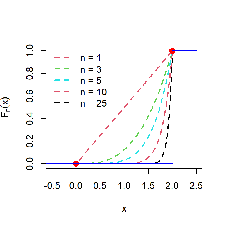
In the light of the above example, let us formalize the concept of the convergence in distribution.
A sequence of random variables \(X_n\) defined on some probability space \((\mathcal{S}, \mathcal{B},\mbox{P})\) with CDF \(F_n(x)\) is said to converge to distribution to another random variable \(X\) having CDF \(F_X(x)\), if the following holds \[\lim_{n\to\infty} F_n(x) = F_X(x)\] at all points \(x\) where the function \(F_X(x)\) is continuous.
An important point to be noted here that for checking the convergence in distribution, we need to check on the convergence at all the points where the function \(F_X(x)\) is continuous.
Let us now see another example of the convergence in distribution. Suppose that \[X_n \sim \sqrt{n}\times \mbox{Uniform}\left(0, \frac{1}{n}\right).\] Let \(U_n \sim \mbox{Uniform}\left(0,\frac{1}{n}\right)\) and then \(X_n = \sqrt{n}\times U_n\).
Therefore, \(X_n\) is basically a product of two components, one is exploding as \(n\to \infty\) and another component is shrinking as \(n\to \infty\).
\[f_{U_n}(x) = \begin{cases}n, 0<x<\frac{1}{n}\\ 0, \mbox{otherwise} \end{cases}\]
\[F_{U_n}(x) = \begin{cases}0, -\infty <x<0 \\ nx, 0\le x<\frac{1}{n}\\ 1, \frac{1}{n}\le x <\infty \end{cases}\]
par(mfrow = c(1,2))
n = 1
f_n = function(x){
  n*(0<x)*(x<1/n)
}
curve(f_n(x), 0, 1, lwd = 2, col = n, ylim = c(0,11),
      lty = 2, ylab = expression(f[n](x)))
n_vals = c(3,5,8,10)
for(n in n_vals){
  curve(f_n(x), add = TRUE, lwd = 2, col = n, lty = 2)
}
legend("topright", legend = c("n = 1", "n = 3", "n = 5", "n = 8", "n = 10"),
       col= c(1,n_vals), bty = "n", lwd = 2, lty = rep(2,5))

F_n = function(x){
  n*x*(0<x)*(x<1/n) + (1/n<=x)
}
n = 1
curve(F_n(x), lwd = 2, col = n, -0.1, 1.1,
      lty = 2, ylab = expression(F[n](x)))
n_vals = c(3,5,8,10)
for(n in n_vals){
  curve(F_n(x), add = TRUE, lwd = 2, col = n, lty = 2)
}
legend("bottomright", legend = c("n = 1", "n = 3", "n = 5", "n = 8", "n = 10"),
       col= c(1,n_vals), bty = "n", lwd = 2, lty = rep(2,5))
segments(-0.1,0, 0,0, col = "blue", lwd = 3)
segments(0,1, 1.5,1, col = "blue", lwd = 3)
points(0,1, pch = 19, col = "blue", cex = 1.2)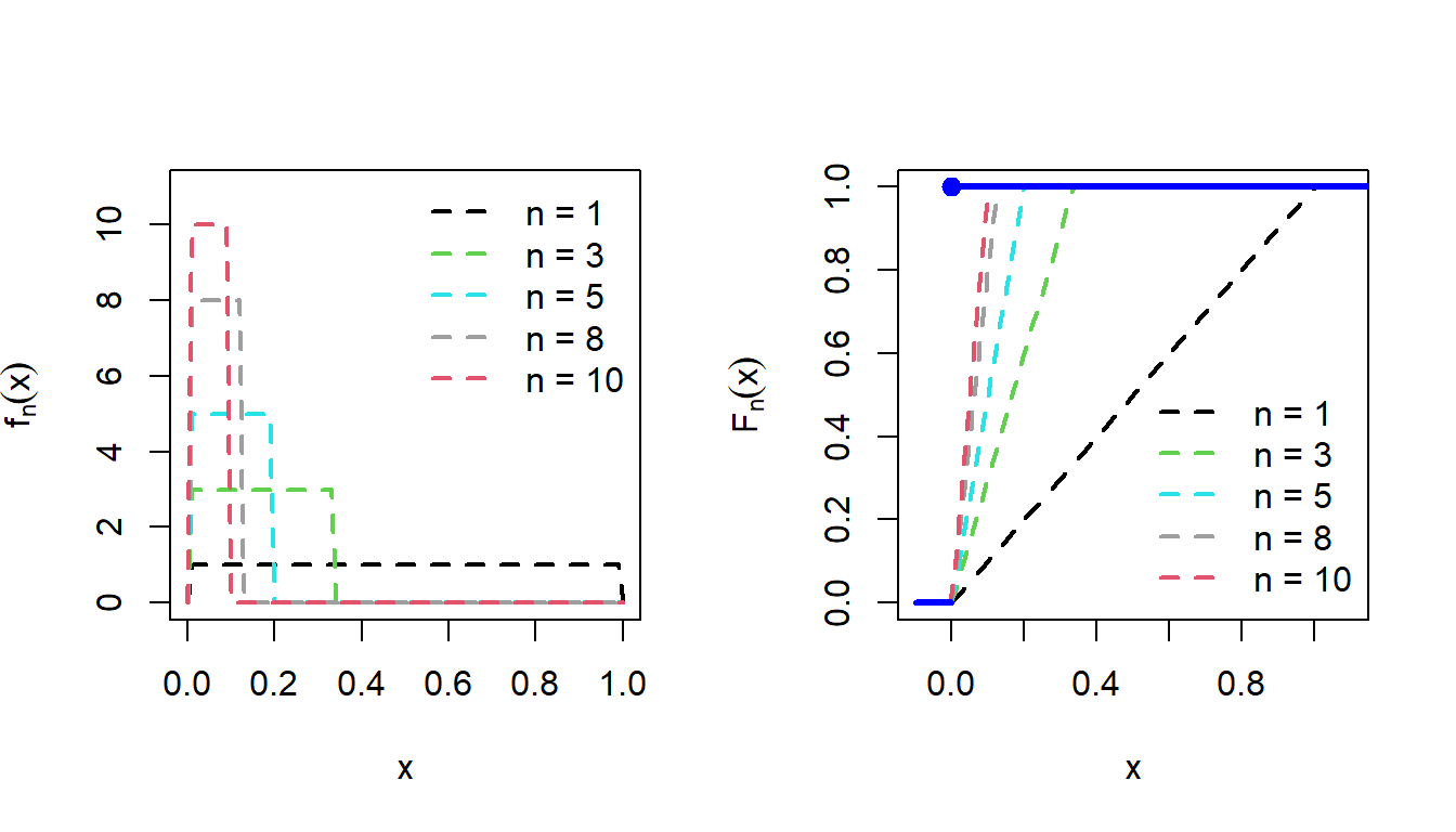
Therefore, \(U_n\) converges in distribution to \(0\) and we are now ready to check that if we multiply \(\sqrt{n}\) with \(U_n\), will it still go to zero? In the following let us consider the simulation of \(U_n\) for different values of \(n\) and also compute \(X_n\) and see how these simulated numbers behave as \(n\to \infty\).
n = 1000
U_n = numeric(length = n)
for(i in 1:n){
  U_n[i] = runif(n = 1, min =0, max = 1/i)
}
plot(1:n, U_n, xlab = "n", type = "l", col = "blue",
     lwd = 2, ylab = " ")
X_n = numeric(length = n)
for(i in 1:n){
  X_n[i] = sqrt(i)*U_n[i]
}
lines(1:n, X_n, col = "red", lwd = 2)
legend("topright", legend = c(expression(U[n]), expression(X[n])),
       col = c("blue", "red"), lwd = c(2,2), bty = "n")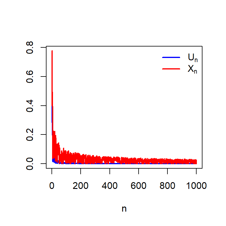
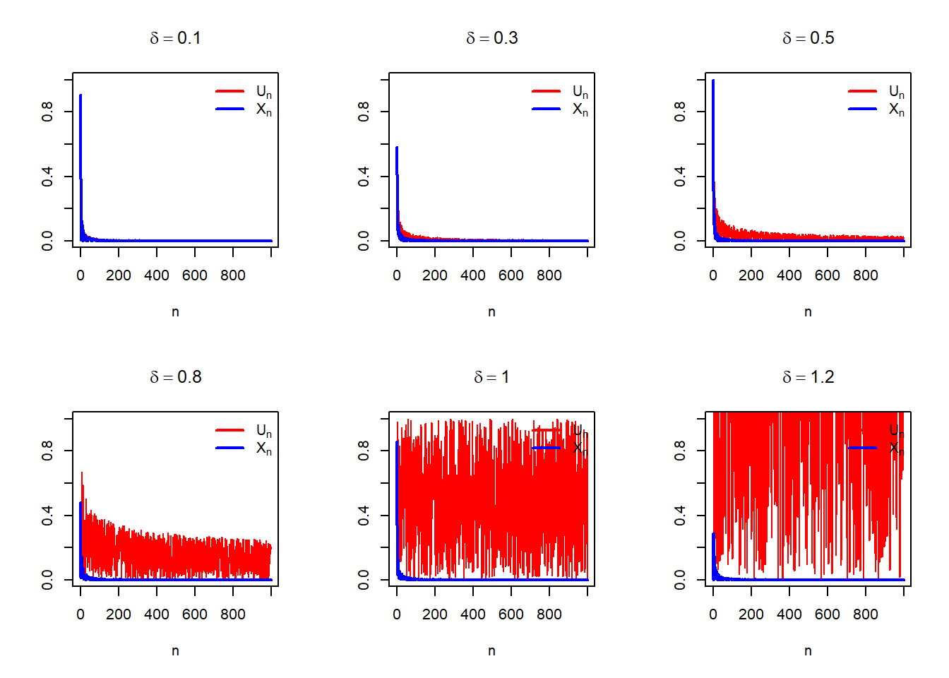
We can expand the scope of this problem by expanding the definition of \(X_n\) as follows: \[X_n = n^{\delta}U_n, \delta>0.\] In the following, we choose different values of \(\delta\) and see how to simulations behave. The following simulations suggest that
delta_vals = c(0.1, 0.3, 0.5, 0.8, 1, 1.2)
par(mfrow = c(2,3))
for(delta in delta_vals){
  n = 1000
  U_n = numeric(length = n)
  for(i in 1:n){
    U_n[i] = runif(n = 1, min =0, max = 1/i)
  }
  X_n = numeric(length = n)
  for(i in 1:n){
    X_n[i] = i^delta*U_n[i]
  }
  plot(1:n, X_n, xlab = "n", ylab = "",
     type = "l", col = "red", main = bquote(delta == .(delta)),
     ylim = c(0,1))
  lines(1:n, U_n, col = "blue", pch = 19, lwd = 2)
  legend("topright", legend = c(expression(U[n]), expression(X[n])),
         col = c("red", "blue"), lwd = c(2,2),
         bty = "n")
}
We have learnt two different convergence concepts: Convergence in probability and the convergence in distribution. In notation they are denoted as \[X_n \overset{P}{\to} X,~~~~X_n \overset{d}{\to} X.\] The following results hold:
If \(X_n \overset{P}{\to} X\), then \(X_n \overset{d}{\to} X\). The converse of the statement is not true in general. However, if \(X_n \overset{P}{\to} X\) and \(X\) is a degenerate random variable (that is a constant), then \(X_n \overset{P}{\to} X\) as well.
If \(X_n \overset{P}{\to} X\) and \(Y_n \overset{P}{\to} Y\), then \(X_n+Y_n \overset{P}{\to} X+Y\).
If \(X_n \overset{P}{\to} X\) and \(a\) is a real number, then \(aX_n \overset{P}{\to} aX\).
If \((a_n)\) be a sequence of real numbers with \(a_n\to a\) as \(n\to \infty\) and \(X_n \overset{P}{\to} X\), then \(a_nX_n \overset{P}{\to} aX\).
Suppose that we have a random sample of size \(n\) from the population distribution whose PDF of PMF is given by \(f(x)\). In addition, assume that the population has finite variance \(\sigma^2<\infty\). Let \(\mu = \mbox{E}(X)\) be the population mean. We denoted the sample mean using the symbol \(\overline{X_n}= \frac{1}{n}\sum_{i=1}^n X_i\). Due to the WLLN, we have observed that \(\overline{X_n}\to \mu\) in probability as \(n\to\infty\). It is to be noted that for every \(n\ge 1\), \(\overline{X_n}\) is a random variable and depending on the problem, its exact probability distribution may be computed. For example, if \(X_1,X_2,\ldots,X_n\) be a random sample of size \(n\) from the normal distribution with mean \(\mu\) and variance \(\sigma^2\), then \[\overline{X_n}\sim\mathcal{N}\left(\mu, \frac{\sigma^2}{n}\right), \mbox{ for all }n\ge 1.\] One can show that the MGF of \(\overline{X_n}\) is given by \[M_{\overline{X_n}}(t) = e^{\mu t + \frac{1}{2}\frac{\sigma^2}{n}t}, -\infty<t<\infty.\] which establishes the result by the uniqueness of the MGF.
Now can we generalize this result for any population distribution with finite variance? In particular, can for large sample size \(n\), the sampling distribution of \(\overline{X_n}\) be approximated by some normal distribution? If so, what will be the mean and variance of the approximating normal distribution?
Before going to provide an exact answer of the above questions, let us perform some computer simulations and see how the sampling distribution of the sample mean behaves for large sample size \(n\) and for different population distributions.
In the following code, we repeatedly simulate a sample of size \(n\) from the exponential distribution with rate \(\lambda\), which is given by \[f_X(x)=\begin{cases}\lambda e^{-\lambda x},~ 0<x<\infty\\ 0, ~~~~~~~~~\mbox{otherwise}\end{cases}.\] The distribution is positively skewed and does not have any apparent connection with the normal distribution. We implement the following algorithm:
lambda = 2
n_vals = c(3,5,10,25,50,100)
rep = 1000
par(mfrow = c(2,3))
for(n in n_vals){
  sample_mean = numeric(length = rep)
  for(i in 1:rep){
    x = rexp(n = n, rate = lambda)
    sample_mean[i] = mean(x)
  }
  hist(sample_mean, probability = TRUE, breaks = 30,
       xlab = expression(bar(x)), main = paste("n = ", n))
  curve(dnorm(x, mean = 1/lambda, sd = sqrt(1/(lambda^2*n))),
        add = TRUE, col = "red", lwd =2)
  curve(dgamma(x, shape = n, rate = lambda*n),
        col = "blue", lwd = 3, lty = 2, add = TRUE)
}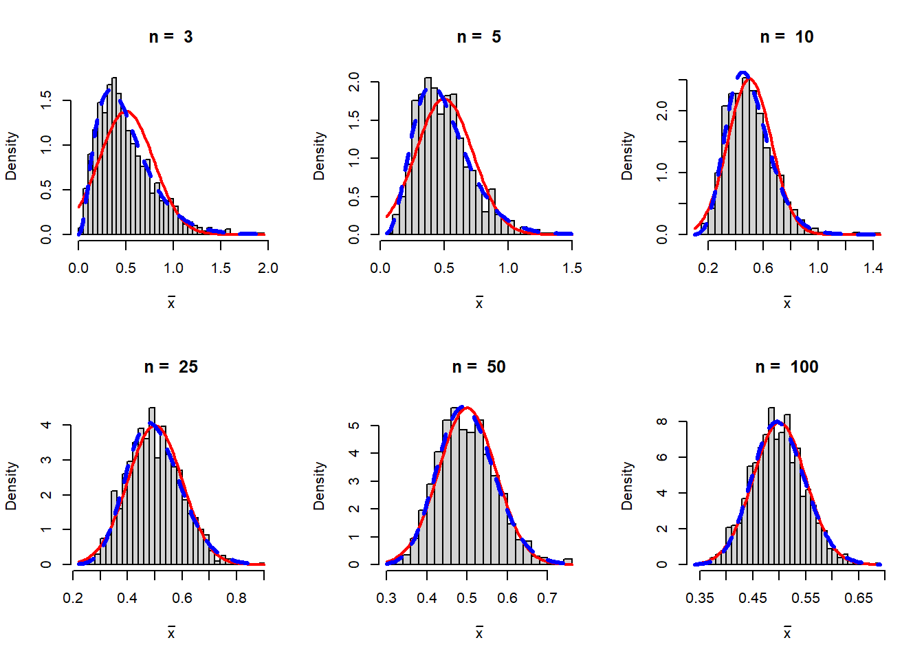
In this simulation study we are lucky that the exact sampling distribution of the sample mean \(\overline{X_n}\) can be derived using the MGF. The sampling distribution is given by
\[f_{\overline{X_n}}(x)= \begin{cases}\frac{(n\lambda)^ne^{-n\lambda x}x^{n-1}}{\Gamma(n)}, 0<x<\infty\\ 0, ~~~~~~~~~~~~~~~~~~~~\mbox{otherwise} \end{cases}.\]
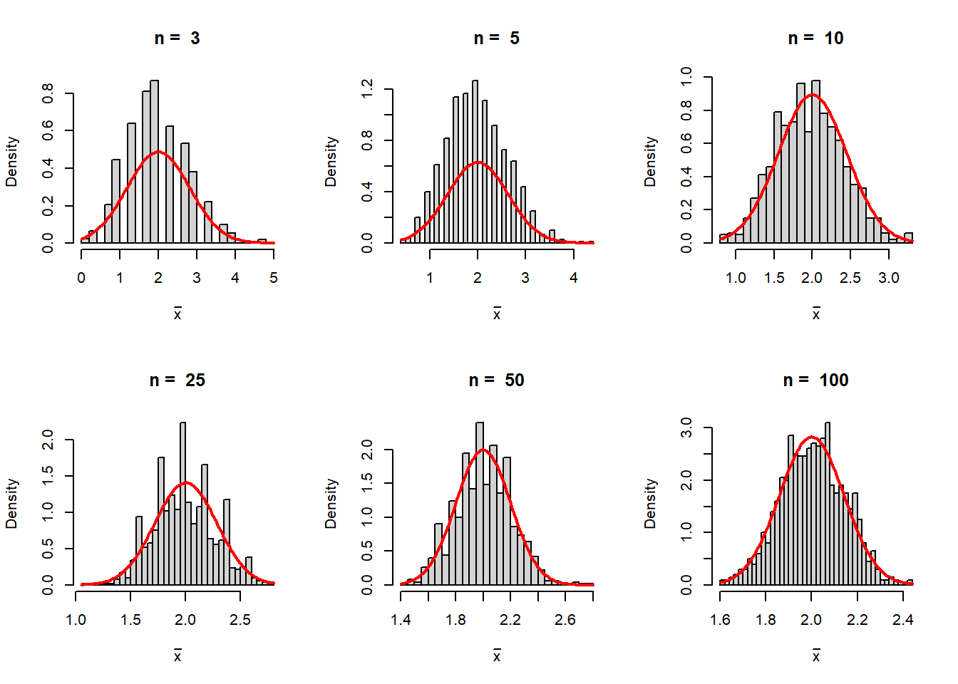
We repeat the above simulation exercise for the Poisson distribution with rate \(\lambda\). In the resulting histograms we overlay the normal distribution with mean \(\lambda\) and variance \(\frac{\lambda}{n}\).
lambda = 2
par(mfrow = c(2,3))
n_vals = c(3, 5, 10, 25, 50, 100)
rep = 1000
for(n in n_vals){
  sample_mean = numeric(length = rep)
  for(i in 1:rep){
    x = rpois(n = n, lambda = lambda)
    sample_mean[i] = mean(x)
  }
  hist(sample_mean, probability = TRUE, breaks =30,
       xlab = expression(bar(x)), main = paste("n = ", n))
  curve(dnorm(x, mean = lambda, sd = sqrt(lambda/n)),
        add = TRUE, col = "red", lwd =2)
}
A natural question arises that whether for all probability distributions, the Central Limit Theorem holds. The answer is negative. Let us have a simulation experiment using the standard Cauchy distribution which is given by
\[f(x)=\frac{1}{\pi(1+x^2)}, -\infty<x<\infty.\]
par(mfrow = c(1,3))
curve(dcauchy(x), -5, 5, col = "red", lwd = 2)
curve(dnorm(x), add = TRUE, col = "blue", lwd = 2)

n_vals = 1:1000
sample_mean = numeric(length = length(n_vals))
for(n in n_vals){
  sample_mean[n] = mean(rcauchy(n = n))
}
plot(n_vals, sample_mean, col = "red", lwd = 2,
     type = "l", xlab = "sample size (n)")

n = 500
M = 1000
sample_mean = numeric(length = M)
for(i in 1:M){
  sample_mean[i] = mean(rcauchy(n = n))
}
hist(sample_mean, probability = TRUE,
     main = paste("n = ", n))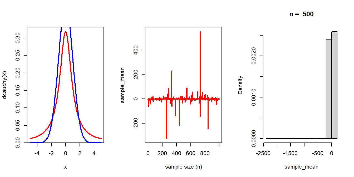
Based on our discussion, we conclude the following:
A further generalization of the CLT led us investigate the sampling distribution of the function of sample mean, \(g\left(\overline{X_n}\right)\) for some function \(g(\cdot)\). For reasonable choice of the function, can we have some large sample approximation of the sampling distribution of \(g\left(\overline{X_n}\right)\)?
The Weak Law of Large Numbers is often used in the computation of numerical integration. The idea is to express the integral as the expected value of a function of a random variable. This expected value is then approximated by averaging the appropriate transformation of the sample values. Let us consider a simple example of integrating the function \(g(x) = e^{-x^2}\) in the interval \((0,1)\). Let us denote the integral as \[I = \int_0^1 e^{-x^2}.\] Certainly the integral is very simple to compute numerically and we can get its value also using the following code:
g = function(x){
  exp(-x^2)
}
integrate(g, 0, 1)
0.7468241 with absolute error < 8.3e-15Suppose that we take a strategy to write down this integral as an expected value of a function as follows: \[I = \int_0^1 e^{-x^2} dx = \int_{-\infty}^{\infty}e^{-x^2} (f_m(x))^{-1}f_m(x)dx = \mbox{E}_{X\sim f_m}\left(e^{-X^2}(f_m(X))^{-1}\right)\] where \(f_m(x)\) is a probability density function for each \(m\in\{1,2,\ldots\}\) defined by \[f_m(x) = \begin{cases} mx^{m-1}, 0<x<1, \\ 0, ~~~\mbox{otherwise}. \end{cases}\] It is easy to follow that \(f_1(x)\) is basically the uniform distribution over \((0,1)\). Let us first consider the case \(m=1\). Therefore, we simulate random numbers \(X_1, \ldots,X_n \sim \mbox{Uniform}(0,1)\) and compute the average of \(e^{-X_1^2}, \ldots,e^{-X_n^2}\), \(\frac{1}{n}\sum_{i=1}^n e^{-X_i^2}\) which is an estimate of \(I\), call it \(\widehat{I_n}\). By WLLN \(\widehat{I_n} \to I\), in probability.
n = 1000
x = runif(n)
I_n = mean(exp(-x^2))
print(I_n)                # Monte Carlo approximate of I
[1] 0.7557172It is clear that \(\widehat{I_n}\) is quite close to \(I\) and as \(n\) increases it becomes more close to \(I\). Students are encouraged to write a code for a visual demonstration of this fact.
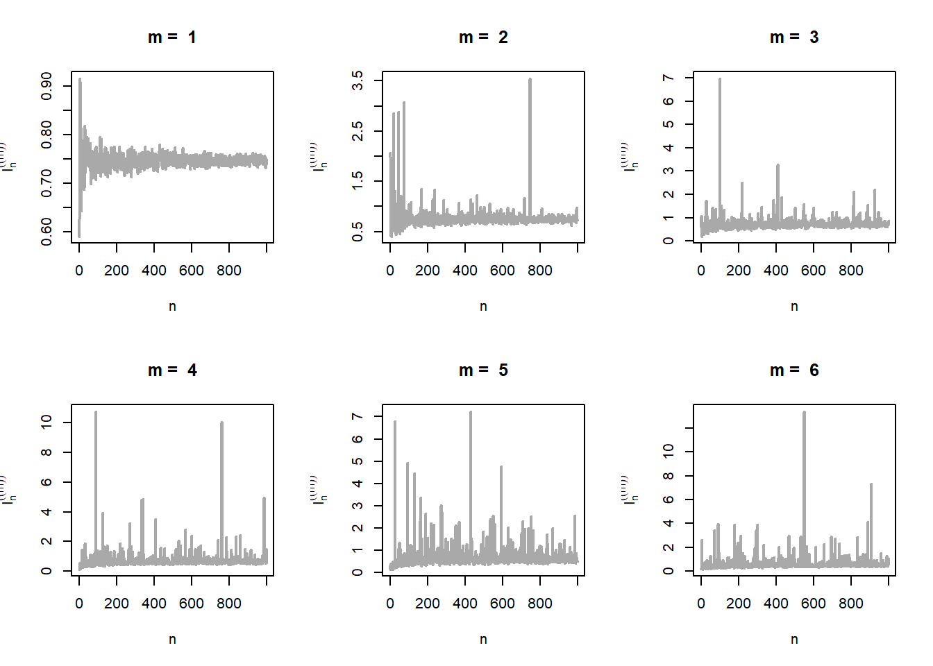
Now suppose that instead of uniform distribution, that is for \(m=1\), we would like to try for different values of \(m\) as well. We call \[\psi_m(x) = \frac{1}{m}e^{-x^2}x^{1-m}, 0<x<1\] and zero otherwise, and \(m\in \{1,2,\ldots\}\). We simulate \(X_1,\ldots,X_n \sim f_m(x)\) and compute \[\widehat{I_n^{(m)}} = \frac{1}{n}\sum_{i=1}^n \psi_m(X_i).\] In the following, we utilize the probability integral transform to simulate the observations from \(f_m(x)\). The CDF of \(f_m(x)\) is given by \[F_m(x) = \begin{cases} 0, ~~~~~x\le 0, \\ x^m, ~~0<x\le 1 \\ 1,~~~~1<x<\infty \end{cases}\] If \(U\sim \mbox{Uniform}(0,1)\), then \(X = U^{1/m}\sim f_m(x)\). Students are encouraged to run the following codes and check on their own.
f_m = function(x){
  m*x^(m-1)*(0<x)*(x<1)
}
m = 2
n = 100
u = runif(n = n)
x = u^(1/m)
hist(x, probability = TRUE, main = paste("m = ", m))
curve(f_m(x), add = TRUE, col = "red", lwd = 2)
In the following we see how the sequence \(I_n^{(m)}\) converges to \(I\) for different choices of \(m\) as \(n\to \infty\).
par(mfrow = c(2,3))
f_m = function(x){              # the PDF
  m*x^(m-1)*(0<x)*(x<1)
}
psi_m = function(x){            # psi function g(x)/f_m(x)
  (1/m)*exp(-x^2)*x^(1-m)
}
n_vals = 1:1000                # n values
m_vals = c(1,2,3,4,5,6)        # different values of m
for(m in m_vals){
  I_n = numeric(length = length(n_vals))
  for(n in n_vals){
    u = runif(n)               # simulate from uniform(0,1)
    x = u^(1/m)                # probability integral transform
    I_n[n] = mean(psi_m(x))
  }
  plot(n_vals, I_n, col = "darkgrey", lwd = 2, type = "l",
       xlab = "n", ylab = expression(I[n]^((m))),
       main = paste("m = ", m))
}
For different choices of \(m\), we can estimate the standard error associated with the approximation. The estimated standard error associated with Monte Carlo approximation \(\widehat{I_n}\) is given by \(s/\sqrt{n}\), where \(s=\sqrt{\frac{1}{n-1}\sum_{i=1}^n\left(\psi_m(X_i) - \widehat{I_n}\right)^2}\). Let us plot the standard error with respect to different choices of \(m\).
n = 10000
m_vals = 1:9
mat_psi_m = matrix(data = NA, nrow = n, ncol = length(m_vals))
I_n_SE = numeric(length = length(m_vals))
for(m in m_vals){
  set.seed(m+100)
  u = runif(n = n)
  x = u^(1/m)
  I_n = mean(psi_m(x))
  I_n_SE[m] = sd(psi_m(x))/sqrt(n)
  mat_psi_m[ ,m] = psi_m(x)
}
plot(m_vals, I_n_SE, type = "b", pch = 19,
     col = "red", cex = 1.3, xlab = "m", lwd = 2,
     main = expression(SE(I[n]^{(m)})), ylab = "Standard Error")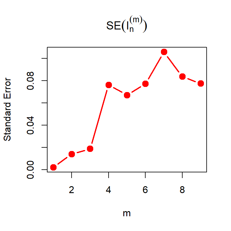
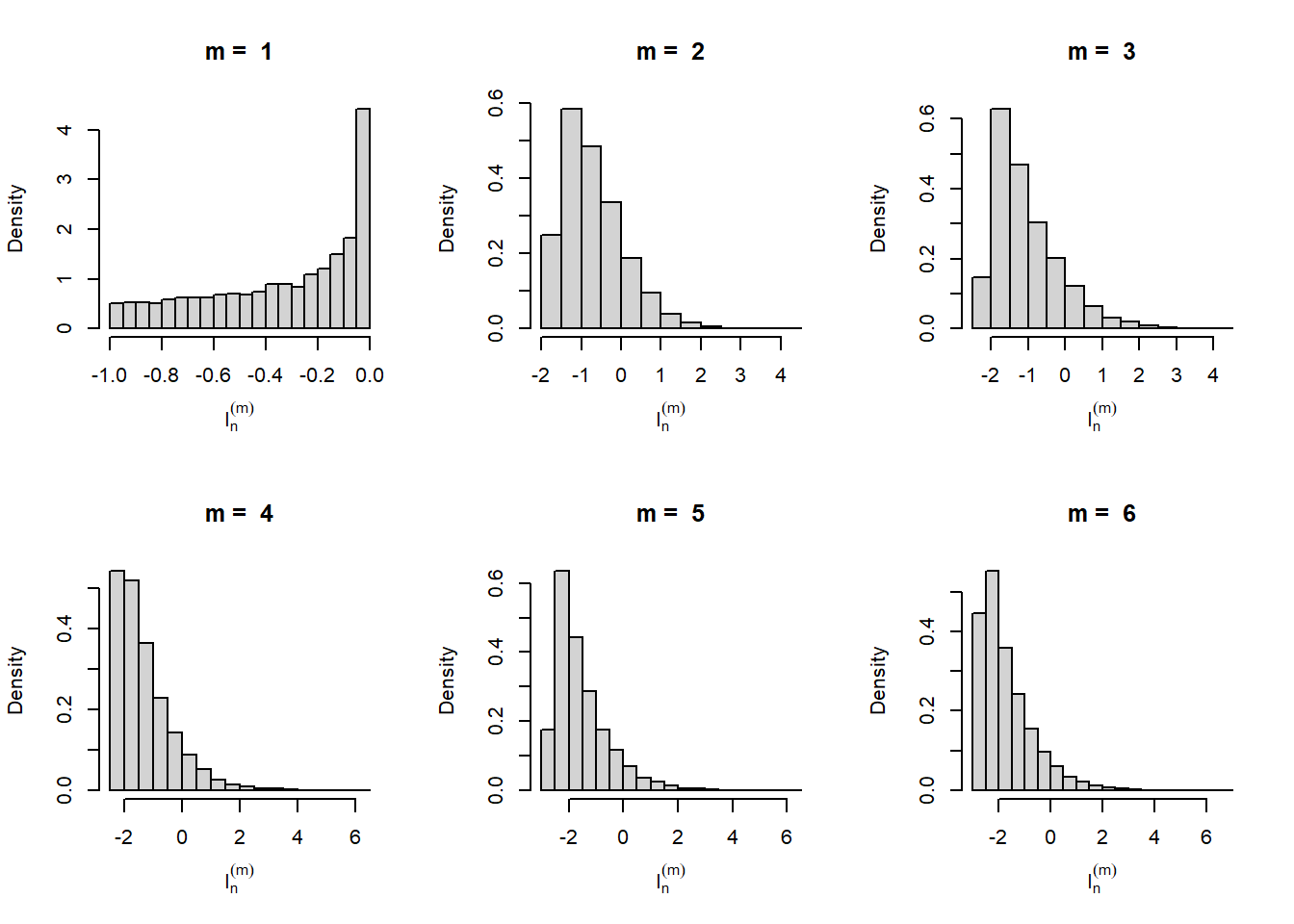
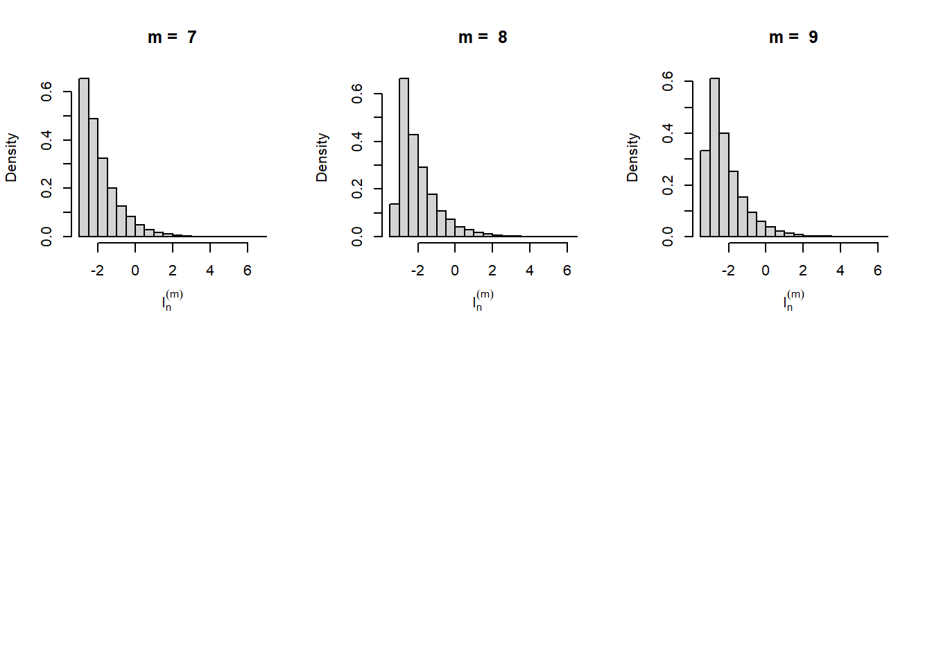
par(mfrow = c(2,3))
for(m in m_vals){
  hist(log(mat_psi_m[,m]), probability = TRUE,
       xlab = expression(I[n]^(m)), main = paste("m = ", m))
}
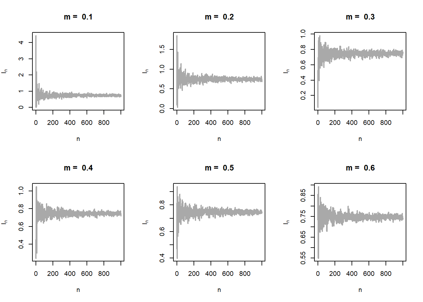
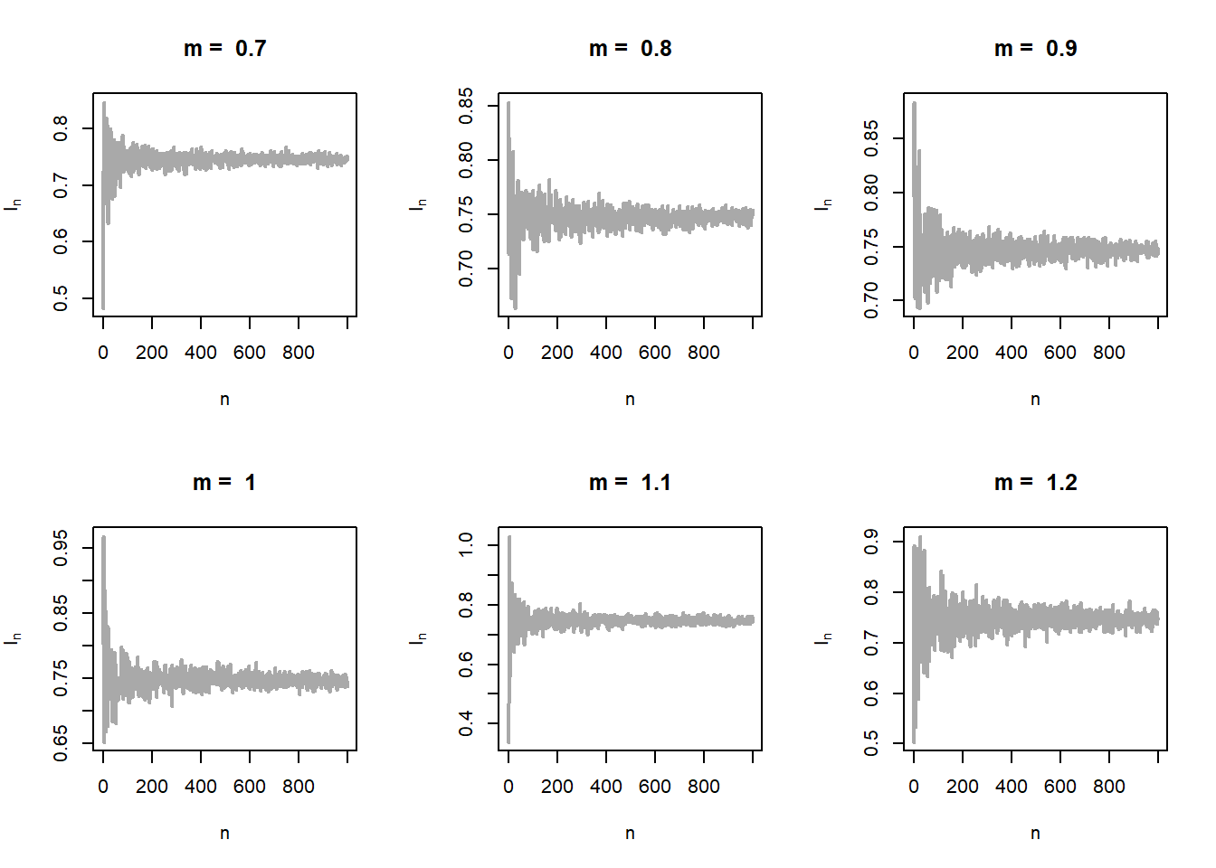
The problem can be generalized further using the fact that \(m\) not necessarily be a positive integer. In fact for any \(m>0\), \(f_m(x)\) is a probability density function. Let us relax this condition for \(m\) and consider an interval of choices for \(m\in(0,2)\) (say). Let us execute the above exercise for real values of \(m\). The shape of the distribution of \(\psi_m(X)\) is shown in Figure 5.23 (left panel). In the right panel of Figure 5.23, the estimated standard error of \(I_n^{(m)}\) has been shown as a function of \(m\). It is evident that there is a moderate value of \(m\) at which the approximation is the best.
par(mfrow = c(2,3))
m_vals = seq(0.1, 1.8, by = 0.1)
n_vals = 1:1000
for(i in 1:length(m_vals)){
  m = m_vals[i]                               # value of m
  I_n = numeric(length = length(n_vals))      # value of psi_m(x_i)
  for(n in n_vals){
    u = runif(n = n)
    x = u^(1/m)
    I_n[n] = mean(psi_m(x))
  }
  plot(n_vals, I_n, main = paste("m = ", m),
       col = "darkgrey", lwd = 2, xlab = "n",
       ylab = expression(I[n]), type = "l")

}
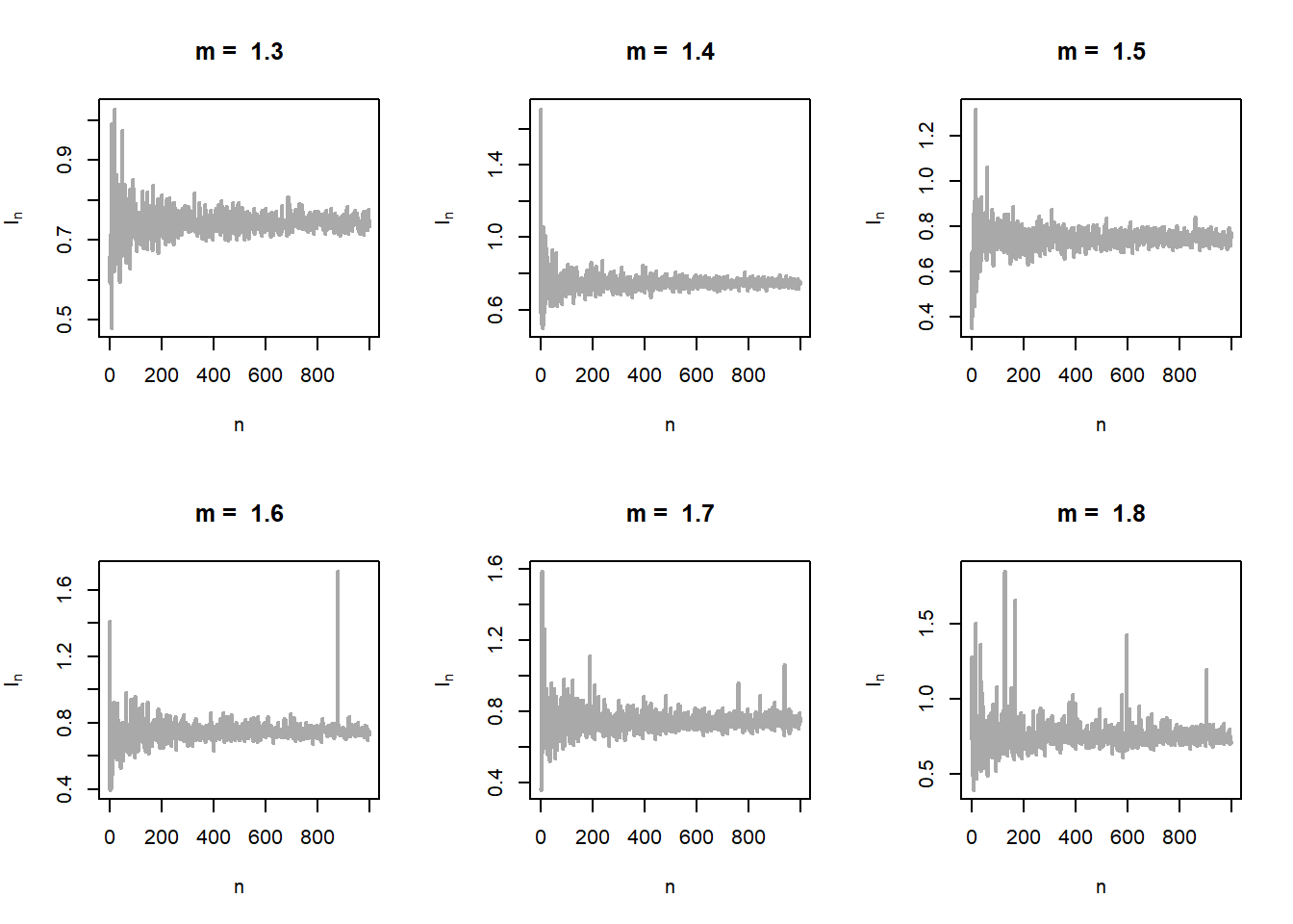
In the following code, let us estimate the standard error associated with the approximation.
par(mfrow = c(1,2))
m_vals = seq(0.1, 1.5, by = 0.08)
n = 1000
mat_psi_m = matrix(data = NA, nrow = n, ncol = length(m_vals))
for(j in 1:length(m_vals)){
  m = m_vals[j]
  u = runif(n = n)
  x = u^(1/m)
  mat_psi_m[, j] = psi_m(x)
}
boxplot(mat_psi_m, names = m_vals)
plot(m_vals, apply(mat_psi_m, 2, sd)/sqrt(n), type = "b",
     col = "red", lwd = 2, pch = 19, xlab = "m",
     ylab = "Standard Error", main = expression(SE(I[n]^(m))))
Suppose that we have a random sample of size \(n\) from the Poisson distribution with rate parameter \(\lambda\). We are interested in estimating the probability \(\mbox{P}(X \ge 1)\). In other words, suppose that the number of telephone calls received by a customer in a day is assumed to follow the Poisson distribution with mean \(\lambda\) and we are interested to approximate the probability that the customer will receive at least one call. We know that the MLE of \(\lambda\) is \(\overline{X_n}\), the sample mean. In addition, we have observed some of the important properties of \(\overline{X_n}\).
\(\overline{X_n}\) converges to the population mean \(\lambda\) as \(n\to\infty\) in probability. That is for any \(\epsilon>0\), \(\lim_{n\to\infty}\mbox{P}\left(\left|\overline{X_n}-\lambda\right|>\epsilon\right)=0\). In other words, we also say that \(\overline{X_n}\) is a consistent estimator of \(\lambda\), population mean. This is also followed from the Weak Law of Large Numbers (WLLN) which states that the sample mean converges to the population mean in probability.
Using the Central Limit Theorem, we have also learnt that \[\overline{X_n} \sim \mathcal{N}\left(\lambda, \frac{\lambda}{n}\right),~\mbox{for large }n,\] which states that the sampling distribution of the sample mean can be well approximated by the normal distribution for large sample sizes, when the samples are drawn from a population distribution with finite variance.
In the current problem, the problem is to estimate a function of the parameter \(\lambda\) which is \[\psi(\lambda) = \mbox{P}(X\ge 1) = 1-(1+\lambda)e^{-\lambda}.\] A natural choice is to approximate the parameter \(\psi(\lambda)\) by using \[\psi\left(\overline{X_n}\right) = 1-\left(1+\overline{X_n}\right)e^{-\overline{X_n}}.\] Now our task is to study the behavior of \(\psi\left(\overline{X_n}\right)\), like unbiasedness, consistency and check the asymptotic distribution for large \(n\). Even if we are not able to obtain the exact sampling distribution, but it will be important to check whether we can have some large sample approximations by some known distributions.
By using Taylor’s approximation (first order) about \(\lambda\) and neglecting higher order terms, we can see that \[\psi\left(\overline{X_n}\right)\approx \psi(\lambda) + \left(\overline{X_n}-\lambda\right)\psi'(\lambda).\] Taking expectations on both sides, we see that \[\mbox{E}\left[\psi\left(\overline{X_n}\right)\right] \approx \psi(\lambda).\] This means that \(\psi\left(\overline{X_n}\right)\) is an approximately unbiased estimator of \(\psi(\lambda)\) at least for large \(n\).
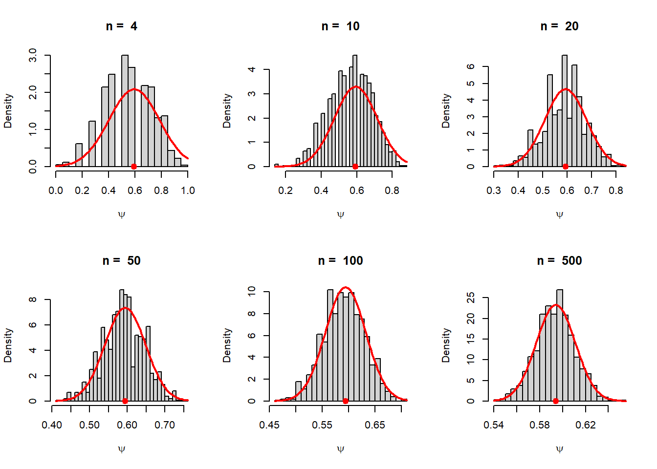
From the above computation, after some rearranging \[\mbox{E}\left(\psi\left(\overline{X_n}\right)-\psi(\lambda)\right)^2 \approx \left(\psi'(\lambda)\right)^2\mbox{E}\left(\overline{X_n}-\lambda\right)^2=\left(\psi'(\lambda)\right)^2Var\left(\overline{X_n}\right)=\frac{\lambda^3e^{-2\lambda}}{n}.\] Therefore, approximate variance of \(\psi\left(\overline{X_n}\right)\) is \(\frac{\lambda^3e^{-2\lambda}}{n}\). In the following simulation, we visualize the sampling distribution of \(\psi\left(\overline{X_n}\right)\).
par(mfrow = c(2,3))
n_vals = c(4, 10, 20, 50, 100, 500)
rep = 1000
lambda = 2
psi = 1-(1+lambda)*exp(-lambda)
for(n in n_vals){
  psi_vals = numeric(length = rep)
  for(i in 1:rep){
    x = rpois(n = n, lambda = lambda)
    psi_vals[i] = 1-(1+mean(x))*exp(-mean(x))
  }
  hist(psi_vals, probability = TRUE,
       xlab = expression(psi), main = paste("n = ", n), breaks = 30)
  points(psi, 0, pch = 19, col = "red", cex = 1.3)
  curve(dnorm(x, mean = psi, sd = sqrt(lambda^3*exp(-2*lambda)/n)), add = TRUE,
        col = "red", lwd =2)
}
For random variables \(X_1,X_2,\ldots,X_n\), show that \[\mbox{E}\left(\sum_{i=1}^n X_i\right) = \sum_{i=1}^n\mbox{E}(X_i)\] and \[Var\left(\sum_{i=1}^n X_i\right)=\sum_{i=1}^n Var(X_i) + 2\sum \sum_{i<j} Cov(X_i,X_j).\]
Let \(X_1,X_2, \ldots,X_n\) and \(Y_1,Y_2,\ldots,Y_m\) be two sets of random variables and let \(a_1,a_2,\ldots,a_n\) and \(b_1,b_2,\ldots,b_m\) be two sets of constants; then prove that \[Cov \left(\sum_{i=1}^n a_iX_i,\sum_{j=1}^m b_jX_j\right) = \sum_{i=1}^n\sum_{j=1}^m a_i b_j Cov\left(X_i,X_j\right)\]
Suppose that \(X_1,X_2,\ldots,X_n\) be a random sample of size \(n\) from a population with PDF \(f(x)\) and CDF \(F(x)\). Define \(Y_1 = \min(X_1,\ldots,X_n)\) and \(Y_n = \max(X_1,X_2,\ldots,X_n)\) be the minimum and the maximum order statistics. Obtain the sampling distribution of \(Y_1\) and \(Y_n\).
Suppose that \(X_1,X_2,\ldots,X_n \sim \mbox{Exponential}(\beta)\) with mean \(\beta\in(0,\infty)\). Obtain the exact sampling distribution of \(Y_1\) and \(Y_n\). Fix \(\beta\) and the sample size \(n\) of your own choice. Simulate a random sample of size \(n\) from the population and obtain the approximate sampling distribution of \(Y_1\) and \(Y_n\) using histograms based on \(m=1000\) replications. Check whether your theoretical derivation matches with the simulation.
Suppose that \(X_1,X_2,\ldots,X_n\) be random sample of size \(n\) from the exponential distribution with mean \(\beta\). Using MGF, obtain the exact sampling distribution of the sample mean \(\overline{X_n}\) and verify your theoretical result using computer simulation.
Suppose that \(X_1,X_2,\ldots,X_n\) be a random sample of size \(n\) from the population distribution whose PDF is given by \(f(x|\theta)=\frac{1}{\theta}, 0<x<\theta\) and zero otherwise. Suppose that we are interested to estimate the parameter \(\theta\) using the sample mean \(\overline{X_n}\). Check whether \(\overline{X_n}\) is an unbiased estimator of \(\theta\). If not can you compute the bias? Also compute the variance of \(\overline{X_n}\). Compute the average squared distance of the estimator from the true value, that is \(\mbox{E}\left(\overline{X_n}-\theta\right)^2\).
Suppose that in the above problem, instead of estimating \(\theta\) using \(\overline{X_n}\), we plan to estimate using the largest order statistics, that is, \(Y_n = \max(X_1,X_2,\ldots,X_n)\). Is it an unbiased estimator of \(\theta\)? Compute the variance of \(Y_n\) and also compute \(\mbox{E}(Y_n-\theta)^2\).
Suppose that \(X_1, X_2, \ldots, X_n\) be a random sample of size \(n\) from the geometric distribution with parameter \(p\), \((0<p<1)\). The population random variable \(X\) represents the number of throws required to get the first success. Starting with uniform random numbers from the interval \((0,1)\), simulate \(n = 30\) realizations from the distribution of \(X\). Suppose that we are interested to estimate \(1/p\) using \(\overline{X_n}\), the sample mean. Based on \(M=10^6\) replications obtain the sampling distribution of \(\overline{X_n}\) and draw the histogram. Do this exercise for \(n \in \{3, 5, 10, 25, 50, 100\}\). Do the histograms shrink as the sample size increases? On each histograms check whether \(\frac{1}{M}\sum_{i=1}^M\overline{X_n}^{(i)}\) is approximately equal to the \(\frac{1}{p}\). What is your conclusion about the unbiasedness of the estimator?