At the beginning of my Statistical Computing lectures, I often share a thought with my students: In statistics, our ultimate goal is to uncover the truth. However, this truth is beyond the reach of humanity—not only now but even in the distant future. When we collect data from natural processes, we aim to understand the workings of nature through mathematical models. Yet, all our efforts based on the collected data merely approximate the true functioning of nature, and achieving 100% accuracy is inherently impossible.
This naturally leads to an important question: If the absolute truth is unattainable, how can we validate statistical approximations and assess their accuracy? This question lies at the very core of understanding the principles and philosophy of statistical science.
However, we need to devise strategies to evaluate how accurate statistical approximations are in estimating the unknown parameters. Suppose that we have a random sample of size \(n\) from the population density function \(f(x;\theta)\) for \(\theta\in \Theta\). We can approximate \(\theta\) based on some function \(\psi(X_1,\ldots,X_n)\), based on a sample of size \(n\). We need to measure the closeness of the estimator \(\psi_n\) to \(\theta\).
6.2 Simulation experiment with Bernoulli distribution
In this section, we approximate the risk function of the sample proportion as an estimator of the true proportion when sampling from the \(\mbox{Bernoulli}(p)\) populations. We perform this task in three steps.
Compute the loss \(\left(\widehat{p_n}- p\right)^2\)
Repeat the following codes multiple times to realize that the loss function \(\mathcal{l}(\widehat{p_n},p)\) is a random variable.
p =0.1# true probabilityn =10# sample sizex =rbinom(n = n, size=1, prob = p) # simulationhead(x)
[1] 0 0 0 0 0 0
pn_hat =mean(x)head(pn_hat)
[1] 0
(pn_hat - p)^2# computing squared loss
[1] 0.01
\(\texttt{Step - II}\)
To compute the average loss, we need to repeat the above process \(M\) times (say) to get an estimate of the risk at a specific value of \(p\).
M =1000# number of replicationpn_loss =numeric(length = M)for(m in1:M){ x =rbinom(n = n, size=1, prob = p) pn_hat =mean(x) pn_loss[m] = (pn_hat - p)^2}head(pn_loss)
\(\texttt{Step - I}\) and \(\texttt{Step - II}\) have been carried out for a fixed value of \(p\). If we want to obtain the performance of the estimator irrespective of the true value, we must evaluate its performance for each \(p\in(0,1)\), which will give us the risk profile of the estimator. This also called a risk function, which is a function of the parameter \(p\) and contain no randomness. \[R(\widehat{p_n},p) = \mbox{E}\left(\mathcal{l}(\widehat{p_n},p)\right).\] We can plot this function as a function of \(p\).
\(\texttt{Step - III}\)
Discretize the parameter space \((0,1)\) into distinct points \(p_1<p_2<\ldots<p_L\).
For each \(p_j, 1\le j\le L\), perform step - I and step - II.
prop_vals =seq(0.01, 0.99, by =0.01)pn_risk =numeric(length =length(prop_vals))M =1000# number of replicationsfor(i in1:length(prop_vals)){ p = prop_vals[i] pn_loss =numeric(length = M)for(m in1:M){ x =rbinom(n = n, size=1, prob = p) pn_hat =mean(x) pn_loss[m] = (pn_hat - p)^2 } pn_risk[i] =mean(pn_loss)}head(pn_risk)
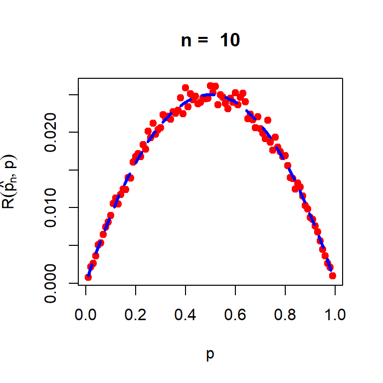
plot(prop_vals, pn_risk, col ="red",pch =19, xlab ="p", ylab =expression(R(hat(p[n]),p)),main =paste("n = ", n))curve(x*(1-x)/(n), add =TRUE, col ="blue", lty =2,lwd =3)
Figure 6.1: The simulated risk function of the MLE of the probability of head \(p\) under the squared error loss. The risk, that is, expected loss has been approximated based on the 1000 replications.
Basically, the risk function says that on an average what will be the mistake in squared error scale, if we replace the true value of \(p\) with the sample proportion.
\(\texttt{Step - IV}\)
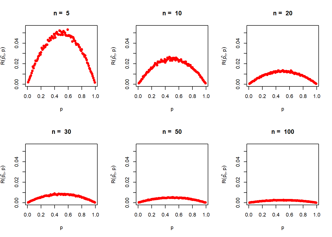
A natural question arises, what will happen if we change the sample size \(n\). Intuition suggests that as \(n\) increases, the distance between the truth and estimate would be small, that \(\mathcal{R}(\widehat{p_n},p)\) would be a decreasing function of \(n\) at each \(p\in (0,1)\). In the following code, we see the behavior of the risk function for different choices of \(p\).
n_vals =c(5, 10, 20, 30, 50, 100)M =1000# number of replicationspar(mfrow =c(2,3))for(n in n_vals){ prop_vals =seq(0.01, 0.99, by =0.01) pn_risk =numeric(length =length(prop_vals))for(i in1:length(prop_vals)){ p = prop_vals[i] pn_loss =numeric(length = M)for(m in1:M){ x =rbinom(n = n, size=1, prob = p) pn_hat =mean(x) pn_loss[m] = (pn_hat - p)^2 } pn_risk[i] =mean(pn_loss) }plot(prop_vals, pn_risk, col ="red",pch =19, xlab ="p", ylab =expression(R(hat(p[n]),p)),main =paste("n = ", n), ylim =c(0,0.055))}
Figure 6.2: The risk function is obtained by using computer simulation based on 1000 replications for different sample sizes \(n\). It is clear that as \(n\to\infty\), te risk goes to zero.
It would be interesting to see whether \(\mathcal{R}\left(\widehat{p_n},p\right)\to 0\) as \(n\to \infty\) for all \(p\in (0,1)\). Theoretical computation can help us in establishing/disproving this claim. The simulated shapes actually supports the theoretical computations as well. The theoretical computation \[\mbox{E}(\widehat{p_n})=\frac{1}{n}\sum_{i=1}^n \mbox{E}(X_i) = \frac{1}{n}np = p.\] Therefore, \[\mbox{E}\left(\overline{X_n}-p\right)^2 = Var_p\left(\overline{X_n}\right) = \frac{1}{n^2}n\times Var(X_1)=\frac{p(1-p)}{n}.\] In the above simulated plots of the risk profiles for different choices of \(n\), you can add the curve \(p(1-p)/n\) and see that the curve is in well agreement is with the simulation.
6.3 Simulation experiment with the normal distribution
Suppose that we have a random sample of size \(n\) from the \(\mathcal{N}(\mu, 1)\) population distribution. We aim to estimate the parameter \(\mu\) using two different estimators \(T_1 = \overline{X_n}\) and \(T_2 = \mbox{Median}(X_1,\ldots,X_n)\).
We are aiming to compare the performance of these two estimators at different values of the unknown parameter \(\mu\). Therefore, we compute \(\mbox{E}\left(T_1 - \mu\right)^2 = R(T_1, \mu)\) and \(\mbox{E}\left(T_2 - \mu\right)^2 = R(T_2, \mu)\).
Consider an interval of \(\mu\) values of your own choice and compute the risk functions using computer simulations and plot them in a single plot window. What is conclusion about the choice of the estimator?
6.4 Sample Mean or Sample Median
n =10sigma =1# fixeda =-1b =1M =1000# number of replicationsmu = ax =rnorm(n = n, mean = mu, sd = sigma)mean(x)
[1] -0.9485205
median(x)
[1] -0.9464891
sample_mean =numeric(length = M)sample_median =numeric(length = M)for(m in1:M){ x =rnorm(n = n, mean = mu, sd = sigma) sample_mean[m] =mean(x) sample_median[m] =median(x)}mean((sample_mean - mu)^2)
[1] 0.09998891
mean((sample_median - mu)^2)
[1] 0.135563
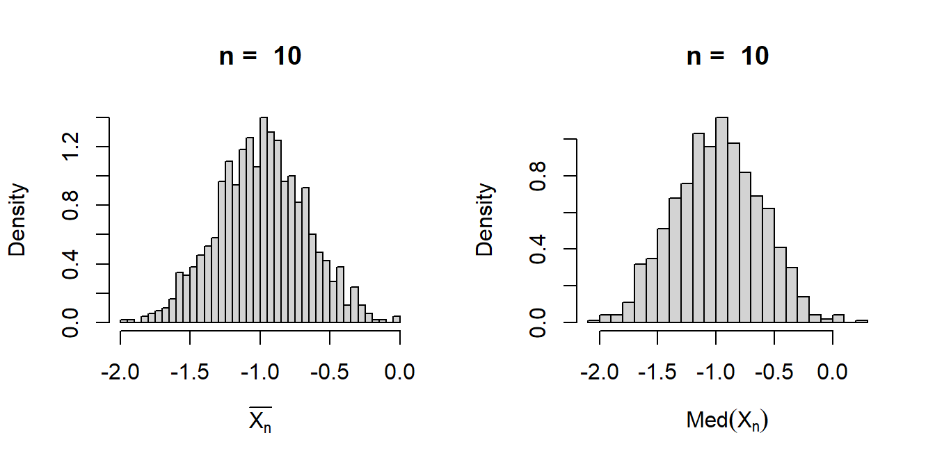
par(mfrow =c(1,2))hist(sample_mean, probability =TRUE, main =paste("n = ", n),breaks =30, xlab =expression(bar(X[n])))hist(sample_median, probability =TRUE, main =paste("n = ", n),breaks =30, xlab =expression(Med(X[n])))
Figure 6.3: The sampling distribution of the sample mean and the sample median have been simulated for sample size \(n=10\) based on 1000 replications. We consider the normal distribution with mean -1 and variance \(1\) for demonstration.
As the value of \(\mu\) changes, we need to check the performance of the sample median and the sample mean.
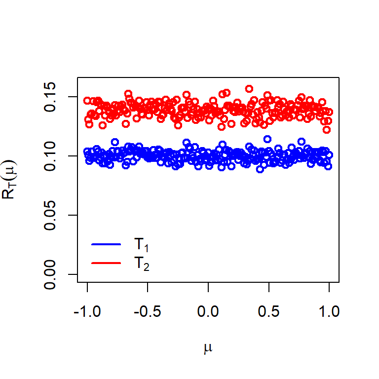
mu_vals =seq(a, b, by =0.01)risk_mean =numeric(length =length(mu_vals))risk_median =numeric(length =length(mu_vals))for (i in1:length(mu_vals)) { sample_mean =numeric(length = M) sample_median =numeric(length = M)for(m in1:M){ x =rnorm(n = n, mean = mu, sd = sigma) sample_mean[m] =mean(x) sample_median[m] =median(x) } risk_mean[i] =mean((sample_mean - mu)^2) risk_median[i] =mean((sample_median - mu)^2)}plot(mu_vals, risk_median, type ="p", col ="red", lwd =2,ylim =c(0, .16), ylab =expression(R[T](mu)), xlab =expression(mu))points(mu_vals, risk_mean, type ="p", col ="blue", lwd =2)legend("bottomleft", legend =c(expression(T[1]), expression(T[2])),col =c("blue", "red"), bty ="n", lwd =c(2,2))
Figure 6.4: The risk values will be constant when the number of replications is large, that is, \(M\to \infty\). From the simulation it is clear that sample mean has uniformly lesser risk than the sample median when used as an etimator for estimating the mean of normally distributed population. Students are encouraged to experiment with this simulation for different values of \(\mu\) and sample size \(n\).
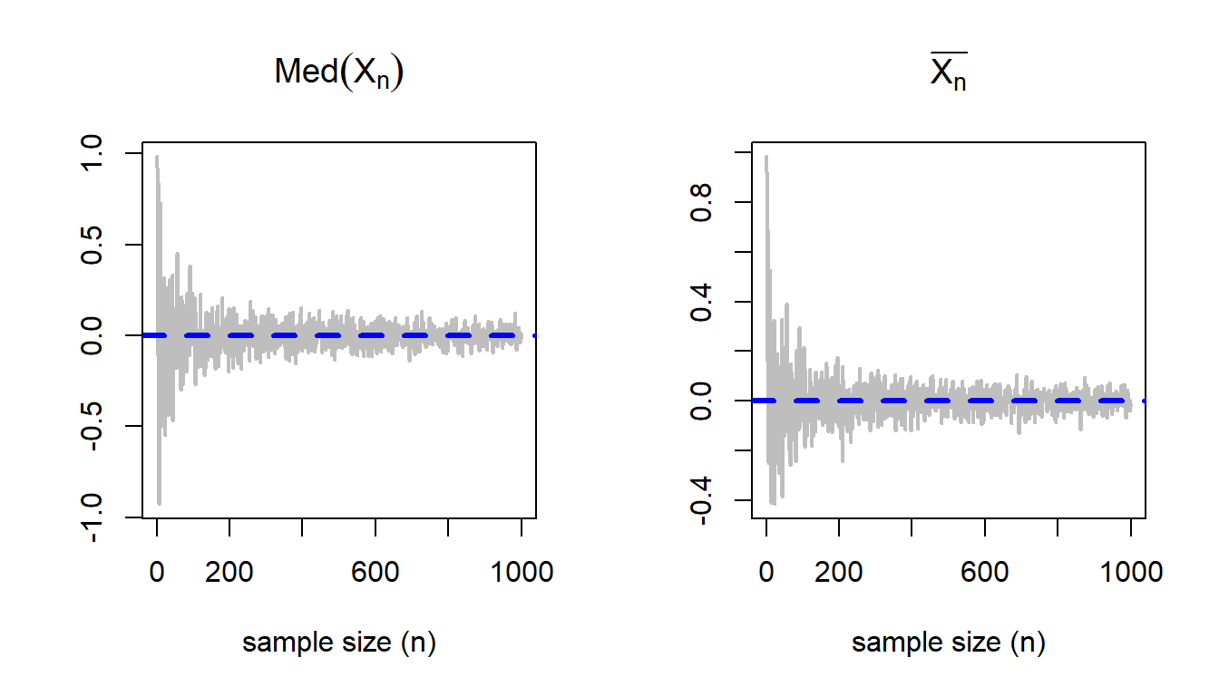
A desirable property of the sample mean and sample median would be to become close to the true value of \(\mu\) as \(n\to \infty\). Using the following visualization, we can check whether these estimators are consistent estimators of the population mean. The following simulation suggests that indeed both of them are consistent, however, fluctuations about the true value is more for the sample median as compared to the sample mean. The following algorithm is implemented to check the consistency.
Plot \(\left(n,\overline{X_n}\right)\) and \(\left(n, \mbox{Med}(X_n)\right)\) for \(n\in\{1,2,\ldots,n_{\mbox{max}}\}\).
n_vals =1:1000mu =0sigma =1sample_median =numeric(length =length(n_vals))sample_mean =numeric(length =length(n_vals))for(n in n_vals){ x =rnorm(n = n, mean = mu, sd = sigma) sample_median[n] =median(x) sample_mean[n] =mean(x)}par(mfrow =c(1,2))plot(n_vals, sample_median, type ="l", col ="grey", lwd =2,xlab ="sample size (n)", main =expression(Med(X[n])),ylab ="")abline(h = mu, col ="blue", lwd =3, lty =2)plot(n_vals, sample_mean, type ="l", col ="grey", lwd =2,xlab ="sample size (n)", main =expression(bar(X[n])),ylab ="")abline(h = mu, col ="blue", lwd =3, lty =2)
Figure 6.5: As the sample size increases, the sample mean and sample median converge to the true value \(\mu\) as \(n\to \infty\).
Asymptotic Comparison of Sample Mean and Sample Median
If \((X_1,X_2,\ldots,X_n)\) be a random sample of size \(n\) from the \(\mathcal{N}(\mu, \sigma^2)\). Then it can be shown that \[\sqrt{n}\left(\overline{X_n}-\mu\right)\overset{D}{\to}\mathcal{N}\left(0,\sigma^2\right)\] and
\[\sqrt{n}\left(\mbox{Med}(X_n)-\mu\right)\overset{D}{\to}\mathcal{N}\left(0,\sigma^2\frac{\pi}{2}\right).\] This result also supports the simulation experiment which showed that both sample mean and sample median converged to the true value of \(\mu\), however, sample median has a larger variance as compared to the sample mean.
6.5 Sample Mean or Sample Variance (Poisson distribution)
To estimate the parameters of the population, the method of moments is a way to obtain estimator(s). In this method, population moments are made equal to the sample moments and the population parameters are expressed as the function of samples.
If the population distribution follows the Poisson distribution with mean \(\lambda\). Then to obtain the MoM estimator of \(\lambda\), we equate the population mean and the sample sample mean \(\overline{X_n}\), which gives the following equation \[\overline{X_n} = \mbox{E}(X) = \lambda.\] Therefore, the MoM moment estimator of \(\lambda\) is \(\overline{X_n}\). However, one can also observe that the population variance is also \(\lambda\) therefore, equating the sample variance \(S_n^2\) with the population variance \((\lambda)\), we find that the sample variance is also an MoM estimator of \(\lambda\). Therefore, the first conclusion is that the Method of Moment estimator is not unique.
A natural question arises, which estimator to prefer in estimating the unknown parameter \(\lambda\)! We have the following observations, \[\mbox{E}\left(\overline{X_n}\right)=\lambda = \mbox{E}\left(S_n^2\right).\] Therefore, both are unbiased estimators of \(\lambda\). We now aproximate the risk functions corresponding to \(\overline{X_n}\) and \(S_n^2\), which are denoted by \(\mathcal{R}\left(\overline{X_n},\lambda\right)\) and \(\mathcal{R}\left(S_n^2,\lambda\right)\), respectively, for \(\lambda\in(0,\infty)\).
In the following
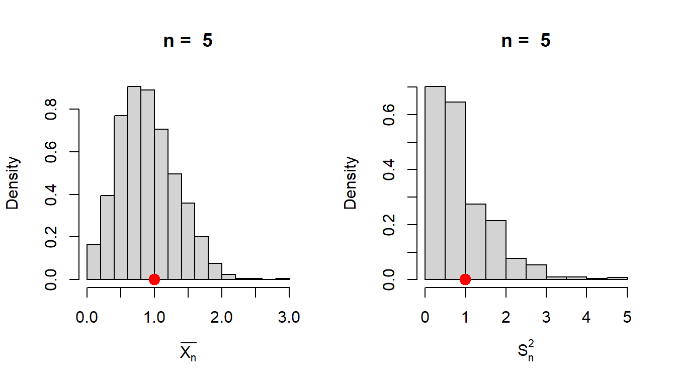
n =5# sample sizeM =1000# number of replicationslambda =1sample_mean =numeric(length = M)sample_var =numeric(length = M)for(i in1:M){ x =rpois(n = n, lambda = lambda) # simulate from Poisson(1) sample_mean[i] =mean(x) sample_var[i] =var(x)}par(mfrow =c(1,2))hist(sample_mean, probability =TRUE,xlab =expression(bar(X[n])), main =paste("n = ",n))points(lambda, 0, pch =19, col ="red", cex =1.5)hist(sample_var, probability =TRUE, main =paste("n = ", n), xlab =expression(S[n]^2))points(lambda, 0, pch =19, col ="red", cex=1.5)# Computing the risk valuesrisk_sample_mean =mean((sample_mean - lambda)^2)cat("The estimated risk the sample mean under squared error loss function is \n",risk_sample_mean)
The estimated risk the sample mean under squared error loss function is
 0.18732
risk_sample_var =mean((sample_var - lambda)^2)cat("The estimated risk of the sample variance under squared error loss function is \n",risk_sample_var)
The estimated risk of the sample variance under squared error loss function is
 0.56925
Figure 6.6: The simulated histograms are obtained based on 1000 replications. The population parameter \(\lambda\) is fixed at \(1\) and the sample size \(n = 5\) is fixed for simulation. The histograms clearly suggests that the spread is more for the sample variance as compared to the sample mean about the true value of \(\lambda\), which is denoted by the red dot.
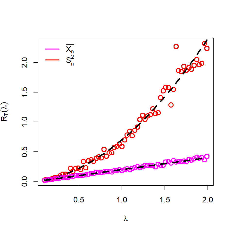
Since, we do not know what is the true value of \(\lambda\), in the following code, we performed the same task at different choices of \(\lambda\). For simulation, purpose, we discretize the \((0.1,3)\) interval for possible choices of \(\lambda\).
n =5M =1000par(mfrow =c(1,1))lambda_vals =seq(0.1, 2, by =0.03)risk_sample_mean =numeric(length =length(lambda_vals))risk_sample_var =numeric(length =length(lambda_vals))for(j in1:length(lambda_vals)){ lambda = lambda_vals[j] sample_mean =numeric(length = M) sample_var =numeric(length = M)for(i in1:M){ x =rpois(n = n, lambda = lambda) sample_mean[i] =mean(x) sample_var[i] =var(x) } risk_sample_mean[j] =mean((sample_mean - lambda)^2) risk_sample_var[j] =mean((sample_var - lambda)^2)}plot(lambda_vals, risk_sample_var, type ="p", col ="red", lwd =2, ylab =expression(R[T](lambda)), xlab =expression(lambda), cex =1.3)lines(lambda_vals,lambda_vals/n +2*lambda_vals^2/(n-1), col ="black",lwd =3, lty =2)points(lambda_vals, risk_sample_mean, type ="p", col ="magenta", lwd =2, cex =1.3)legend("topleft", legend =c(expression(bar(X[n])), expression(S[n]^2)),col =c("magenta", "red"), bty ="n", lwd =c(2,2))lines(lambda_vals, lambda_vals/n, col ="black",lwd =3, lty =2)
Figure 6.7: Approximation of the risk function for the sample mean and sample variance in estimating the parameter \(\lambda\) for the Poisson distribution. It is obvious from the plot that the sample sample mean has a lower risk as compared the sample variance. Therefore, \(\overline{X_n}\) is a better estimator as compared \(S_n^2\), although, both are unbiased estimators of \(\lambda\). The magenta lines indicate the exact risk function obtained by theoretical computation.
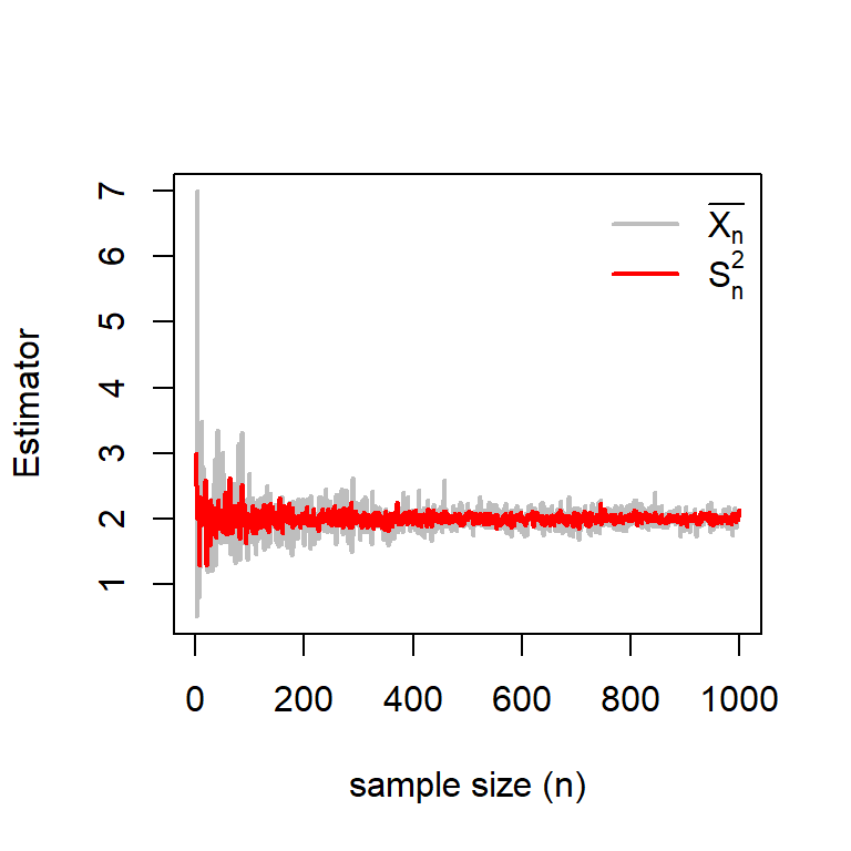
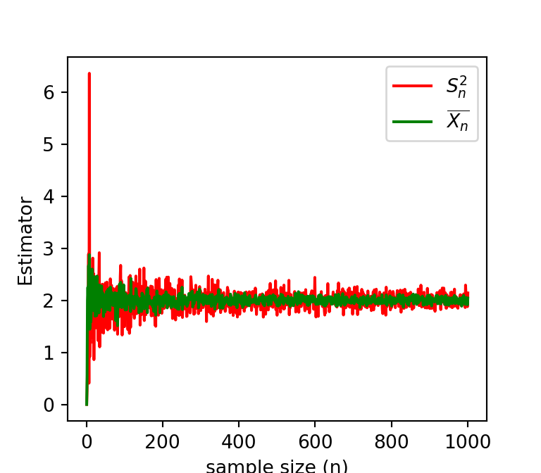
In the classroom, a student named Vaishnavi asked which method would likely converge faster to the true value. The idea is related to the consistency, which means that as \(n\to \infty\), the following claims are true or not. \[\overline{X_n}\overset{P}{\to} \lambda,~~~~~~S_n^2\overset{P}{\to} \lambda\] To answer this question, let us assume that the true value is \(\lambda = \lambda_0 = 2\). We simulate the a sample of size \(n\) from the \(\mbox{Poisson}(\lambda_0)\) and compute \(\overline{X_n}\) and \(S_n^2\) and check how these random quantities behave as \(n\to \infty\). The following code will do this task.
par(mfrow =c(1,1))lambda_0 =2n_vals =1:1000sample_mean =numeric(length =length(n_vals))sample_var =numeric(length =length(n_vals))for(n in n_vals){ x =rpois(n = n, lambda = lambda_0) sample_mean[n] =mean(x) sample_var[n] =var(x)}plot(n_vals, sample_mean, col ="grey", lwd =2,xlab ="sample size (n)", type ="l", ylab ="Estimator")lines(n_vals, sample_var, col ="red", lwd =2)legend("topright", legend =c(expression(bar(X[n])), expression(S[n]^2)),col =c("grey", "red"), lwd =c(2,2), bty ="n")
Figure 6.8: It can be observed that as the sample size increases, the convergence of the Sample variance is much faster as compared to the sample mean to the true value of \(\lambda = 2\).
The following is the python implementation of the above convergence concept. Thanks to Sangeeta for the Python implementation.
import numpy as npimport matplotlib.pyplot as pltlambd_0 =2n_vals = np.linspace(1,1000,num=1000)sample_mean = []sample_var = []for n in n_vals: x = np.random.poisson(lambd_0,int(n)) sample_mean.append(np.mean(x)) sample_var.append(np.var(x))plt.plot(n_vals,sample_var,c="r",label="$S^2_{n}$")plt.plot(n_vals,sample_mean,c="g",label="$\overline {X_{n}}$")plt.legend()plt.xlabel("sample size (n)")plt.ylabel("Estimator")plt.figure(figsize=(1,1))plt.show()
Figure 6.9: It can be observed that as the sample size increases, the convergence of the Sample variance is much faster as compared to the sample mean to the true value of \(\lambda = 2\).
Figure 6.10: It can be observed that as the sample size increases, the convergence of the Sample variance is much faster as compared to the sample mean to the true value of \(\lambda = 2\).
6.5.1 Exact Computation of the variance of \(S_n^2\)
We recall that if we have a random sample of size \(n\) from the a population with mean \(\mu\) and variance \(\sigma^2\). Then \[Var\left(\overline{X_n}\right)=\frac{\sigma^2}{n}.\] In addition, \(S_n^2 = \frac{1}{n-1}\sum_{i=1}^n\left(X_i - \overline{X_n}\right)^2\) is an unbiased estimator of \(\sigma^2\). To compute the variance \(Var(S_n^2)\), we observe that the sample variance can also be expressed as \[S_n^2 = \frac{1}{2n(n-1)}\sum_{i=1}^n\sum_{j=1}^n\left(X_i - X_j\right)^2.\] The following general results hold for all population distributions with finite fourth order moment.
\(\mbox{E}\left(S_n^2\right) = \sigma^2\).
\(Var\left(S_n^2\right)= \frac{1}{n}\left(\mu_4-\frac{n-3}{n-1}\mu_2^2\right)\), where \(\mu_1 = \mbox{E}(X_i)\) and \(\mu_j = \mbox{E}\left(X_i-\mu_1\right)^j, j =2,3,4\).
In addition, the covariance between \(\overline{X_n}\) and \(S_n^2\), \(Cov\left(\overline{X_n},S_n^2\right)\) can also be expressed in terms of \(\mu_1,\mu_2,\mu_3,\mu_4\).
For our problem, the population follows the Poisson distribution with parameter \(\lambda\). Therefore, \(\mbox{E}(S_n^2) = \lambda\). The fourth order central moment for the Poisson distribution: \[\mu_4 = \mbox{E}(X-\lambda)^4= \sum_{i=0}^4 \binom{4}{i}\mbox{E}(X^{4-i})\lambda^i = 3\lambda^2 +\lambda.\] The raw moments \(\mbox{E}(X^i), i=1,2,3,4\), can be computed using the Moment Generating function by taking derivatives and evaluating at \(t=0\). The MGF of Poisson distribution is given by \[M_X(t)=e^{\lambda (e^{t}-1)},-\infty<t<\infty.\]\[\begin{eqnarray}
M_X'(0) &=& \lambda \\
M_X''(0) &=& \lambda^2 + \lambda \\
M_X'''(0) & =& \lambda^3 + 3\lambda^2 + \lambda \\
M_X''''(0) &=& \lambda^4 + 6\lambda^3 + 7\lambda^2 +\lambda
\end{eqnarray}\]
This gives \[\mu_4 = 3\lambda^2 + \lambda.\] Therefore, the variance of \(S_n^2\) is given by \[\begin{eqnarray}
Var(S_n^2) &=& \frac{1}{n}\left(3\lambda^2 + \lambda - \frac{n-3}{n-1}\lambda^2\right)\\
&=&\frac{\lambda}{n}+\frac{2\lambda^2}{n-1}.
\end{eqnarray}\]
In the following R code, we add the analytically computed risk function with the risk function estimated by using simulation. The exact risk function is given by \[\mathcal{R}(S_n^2,\lambda) = \frac{\lambda}{n} + \frac{2\lambda^2}{n-1}, 0<\lambda<\infty.\]
6.5.2 Making this problem more interesting
We found that both \(\overline{X_n}\) and \(S_n^2\) are unbiased estimators of \(\lambda\). However, after comparing the risk functions, we found that \[\mathcal{R}\left(\overline{X_n},\lambda\right)\le \mathcal{R}\left(S_n^2,\lambda\right)\] for all \(\lambda\in(0,\infty)\). We can extend this to a class of estimators defined for every constant \(a\) as follows: \[W_a\left(\overline{X_n},S_n^2\right)=a\overline{X_n}+(1-a)S_n^2.\]
For every \(a\), the estimator \(W_a\) is an unbiased estimator of \(\lambda\). Although \(\overline{X_n}\) is better that \(S_n^2\), is it better than \(W_a\) for all constants \(a\)? In other words, is the following statements true? \[\mathcal{R}\left(\overline{X_n},\lambda\right)=\mathcal{R}\left(W_1,\lambda\right)\le \mathcal{R}\left(W_a,\lambda\right), \mbox{ for all } ~~0<\lambda<\infty.\]
Before getting into some statistical theories that may guide us to determine whether \(\overline{X_n}\) is indeed the best choice, you can plot the risk function of \(\mathcal{R}\left(W_a, \lambda\right), 0<\lambda<\infty\) for different choices of \(a\) using computer simulation. Note that that for \(a=1\) (corresponds to \(\overline{X_n}\)) and \(a=0\) (corresponds to \(S_n^2\)) risk functions are already obtained in the previous section. In addition, check that whether for certain values of \(a\), the risk function falls below \(\mathcal{R}\left(\overline{X_n},\lambda\right)\) for some \(\lambda\) values. In the following, let us try to compute the risk of \(W_a\). \[\begin{eqnarray}
\mathcal{R}(W_a,\lambda)&=& \mbox{E}_{\lambda}(W_a-\lambda)^2 \\
&=& \mbox{E}\left[a\left(\overline{X_n}-\lambda\right) + (1-a)\left(S_n^2-\lambda\right)\right]^2\\
&=& a^2 \mathcal{R}\left(\overline{X_n},\lambda\right)+(1-a)^2 \mathcal{R}\left(S_n,\lambda\right)+2a(1-a)\times \mbox{Cov}\left(\overline{X_n},S_n^2\right)\\
&=& a^2 \frac{\lambda}{n}+(1-a)^2\left(\frac{\lambda}{n}+\frac{2\lambda^2}{n-1}\right)+2a(1-a)\frac{\lambda}{n}
\end{eqnarray}\] To obtain the best choice of \(a\), we need to minimize the risk function as a function of \(a\). The equation \(\frac{d}{da}\mathcal{R}(W_a,\lambda)=0\), gives \(a^* = 1\) and \(\frac{d^2}{da^2}\mathcal{R}(W_a,\lambda)|_{a=1}=\frac{2\lambda^2}{n-1}>0\). Therefore the minimum risk is obtained what \(a=1\), which corresponds to the sample mean \(\overline{X_n}\) for all \(\lambda\in(0,\infty)\).
Therefore, we are able to establish that if we consider the class of estimators \(W_a\) (unbiased) indexed by constant \(a\in \mathbb{R}\), then \(\overline{X_n}=W_1\) is the best estimator in this class when compared with respect to the risk function under the squared error loss.
However, it does not guarantee that the sample mean is the best estimator amongst all estimators of \(\lambda\) existing in this globe. Therefore, we need to develop theories which will be helpful to determine whether the sample mean is indeed THE BEST CHOICE to estimate the unknown parameter \(\lambda\).
A natural extension is to extend the class to any unbiased estimator of \(\lambda\). That is can we claim that for any unbiased estimator \(T_n\) of \(\lambda\), \[\mathcal{R}\left(\overline{X_n},\lambda\right) \le \mathcal{R}\left(T_n,\lambda\right)\] for all \(\lambda \in (0,\infty)\).
6.6 Search for the holy grail (the best estimator)
See Next Chapter (Unbiased Estimation)
6.7 Conceptual Exercises
Suppose that a random sample \((X_1,X_2,\ldots,X_n)\) of size \(n\) from a population which is characterized by the following probability density function: \[f(x)=\begin{cases} \frac{2x}{\theta^2}, ~0<x<\theta \\
0,~~~~\mbox{otherwise}\end{cases},\] where \(\theta \in\Theta = (0,\infty)\) be the parameter space. We are interested in estimating the parameter \(\theta\) based on the given random sample. Let \(Y_n = \max(X_1,X_2,\ldots,X_n)\) be the maximum order statistics and you decided to estimate \(\theta\) using \(Y_n\). Answer the following:
Plot the above PDF for different choices of \(\theta\) in a single plot window. Obtain the CDF of the given PDF and plot the CDF different choices of \(\theta\) in a single plot window. Make a side by side plot using \(\texttt{par(mfrow = c(1,2))}\).
Obtain the exact sampling distribution of \(Y_n\) and write down the both probability density function and the cumulative distribution function of \(Y_n\).
Under the squared error loss function, compute the risk function \(\mathcal{R}\left(Y_n,\theta\right), 0<\theta<\infty\). Also, plot the risk function.
Show that as \(n\to \infty\), \(Y_n \to \theta\) in probability. For a fixed \(\epsilon>0\), compute the limit \(\lim_{n\to \infty} \mbox{P}\left(|Y_n-\theta|>\epsilon\right)\) and show the limit is equal to zero as \(n\to\infty\). Another possibility is to apply some inequality to bound the \(\mbox{P}\left(|Y_n-\theta|>\epsilon\right)\) with constant \(a_n\) which converges to \(0\) as \(n\to \infty\) (Hint: Markov Inequality). Write a computer simulation to visualize that the largest order statistics \(Y_n\) indeed converges to \(\theta\) as \(n\to \infty\).
Compute the expected value of \(Y_n\) and compute the bias of the estimator \(Y_n\), which is given by \[\mbox{Bias}_{\theta}\left(Y_n\right) = \mbox{E}\left(Y_n\right)-\theta, \theta\in(0,\infty).\] Also check whether the bias \(\mbox{Bias}_{\theta}\left(Y_n\right)\) tends to zero as \(n\to \infty\). That means is the estimator is asymptotically unbiased? Compute the value of the constant \(c_n\) so that \[\mbox{E}_{\theta}(c_n Y_n) = \theta \mbox{ for all }\theta \in (0,\infty).\]
Compute the variance of \(Y_n\), which can be computed as \[Var_{\theta}\left(Y_n\right) = \mbox{E}_{\theta}\left(Y_n^2\right)-\left(\mbox{E}_{\theta}(Y_n)\right)^2.\]
Show the following identity holds for all \(\theta \in(0,\infty)\): \[\mathcal{R}\left(Y_n,\theta\right) = \mbox{E}_{\theta}\left(Y_n-\theta\right)^2=Var_{\theta}(Y_n)+\left(\mbox{Bias}_{\theta}(Y_n)\right)^2.\]
Using computer simulation, approximate the risk function \(Y_n\), \(\mathcal{R}(Y_n,\theta), \theta\in(0,\infty)\). The challenge, the reader may find is to simulate from the population distribution as some inbuilt function in R may not be available. To simulate a random number from the given distribution (a) Compute the CDF \(F_X(x)\), (b) Simulate \(U \sim \mbox{Uniform}(0,1)\). (c) Compute \(X = F_X^{-1}(U)\), which is the inverse image of \(U\) under \(F_X\). Then \(X\sim f(x)\). Overlay the analytically computed risk function on the plot of the risk function obtained by computer simulation.
6.8 Another illustrative example
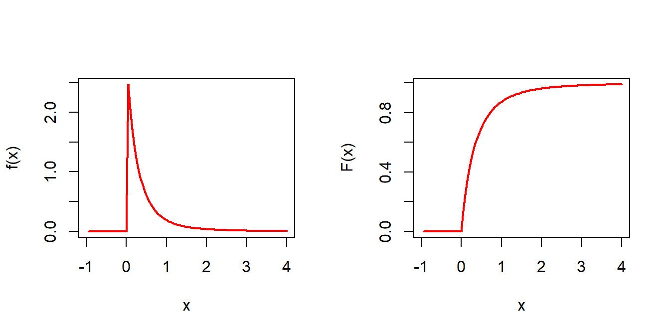
Suppose that we have a sample of size \(n\)\((X_1,X_2,\ldots,X_n)\) from a population which is characterized by the following probability density function and our goal is to estimate the parameter \(\theta \in (0,\infty)\).
\[f(x) = \begin{cases} \frac{\theta}{(1+x)^{1+\theta}}, 0<x<\infty\\
0, ~~~~\mbox{otherwise}
\end{cases}\] At the first step, we compute the cumulative distribution function and plot both PDF and CDF for different choices of \(\theta\) values.
Figure 6.11: The PDF and CDF of the population random variable \(X\) is shown. The value of \(\theta=3\) is considered. The reader is encouraged to modify the R codes to draw different shapes for different choices of \(\theta\) values.
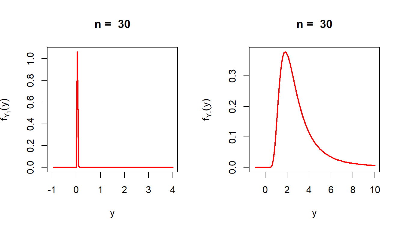
Suppose one starts with the maximum and minimum order statistics to estimate the parameter \(\theta\), which are defined as \(Y_n = \max(X_1,\ldots,X_n)\) and \(Y_1 = \min(X_1,X_2,\ldots,X_n)\). First of all, we compute the sampling distribution of \(Y_1\) and \(Y_n\) and plot the PDFs. \[f_{Y_1}(y) = \begin{cases} n\theta (1+y)^{-(n\theta+1)}, 0<y<\infty,\\
0, \mbox{otherwise.}\end{cases}\]
par(mfrow =c(1,2))n =30f_Y1 =function(x){ (n*theta*(1+x)^(-n*theta-1))*(x>0)}curve(f_Y1(x), -1, 4, col ="red", lwd =2, main =paste("n = ",n),ylab =expression(f[Y[1]](y)), xlab ="y")f_Yn =function(x){ n*((1-(1+x)^(-theta))^(n-1))*theta/(1+x)^(1+theta)*(x>0)}curve(f_Yn(x), -1, 10, col ="red", lwd =2, main =paste("n = ",n),ylab =expression(f[Y[n]](y)), xlab ="y")
Figure 6.12: The sampling distribution of the \(Y_1\) and \(Y_n\). The value of \(\theta\) is set to \(3\). It is clear that \(Y_1\) is highly concentrated at \(0\) and the concentration increases as \(n\) becomes large. Therefore, \(Y_1\) does not appear to be a good choice for estimating \(\theta\). The sample size is fixed at \(n=30\).
One may probably think of using the maximum order statistics \(Y_n = \max(X_1, X_2, \ldots,X_n)\) to estimate the parameter \(\theta\). Let us investigate the properties of the estimator \(Y_n\). At the first step we can compute the mean and higher order moments of \(Y_n\).
The mean of \(Y_n\) can be computed by computing the expectation of \(Y_n+1\) as follows: \[\begin{eqnarray}
\mbox{E}_{\theta}(Y_n+1) &=& \int_0^{\infty}(1+y)n\left[1-(1+y)^{-\theta}\right]^{n-1}\cdot \frac{\theta}{(1+y)^{1+\theta}}dy \\
& =& n\mathcal{B}\left(1-\frac{1}{\theta},n\right), \theta\in(1,\infty)\end{eqnarray}\]
The expectation exists only when \(\theta\in(1,\infty)\). More importantly, \(\mbox{E}(Y_n) \ne \theta\), therefore, \(Y_n\) is not an unbiased estimator of \(\theta\). A similar computation will give us \(\mbox{E}_{\theta}\left(Y_n+1\right)^2 = n\mathcal{B}\left(1-\frac{2}{\theta},n\right), \theta\in(2,\infty)\). The above result can be generalized as
\[\begin{eqnarray}
\mbox{E}_{\theta}(Y_n+1)^m &=& \int_0^{\infty}(1+y)^m \cdot n\left[1-(1+y)^{-\theta}\right]^{n-1}\cdot \frac{\theta}{(1+y)^{1+\theta}}dy \\
&=& n\mathcal{B}\left(1-\frac{m}{\theta},n\right), \theta\in(m,\infty). \end{eqnarray}\] Then \(m\)th order raw moments exists when \(\theta\in(m,\infty)\). Use the idea of change of variable as \(z = (1+y)^{-\theta}\) to compute the above integrals. Therefore, we can evaluate the risk of \(Y_n\) under the squared error loss as
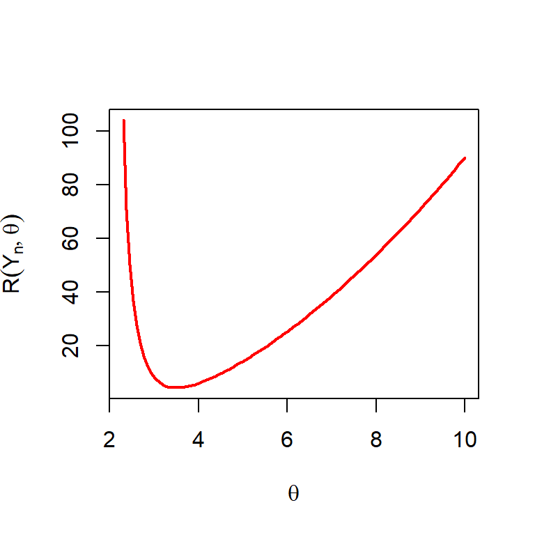
We need to keep in mind that the risk function exists only when \(\theta\in(2,\infty)\). Let us plot the risk function for different choices of \(\theta\). The following figure suggests that the performance of this estimator is reasonable at a small subset of the parameter space.
Figure 6.13: The risk function of \(Y_n\) as a function of \(\theta\). The sample size is fixed at \(n=10\).
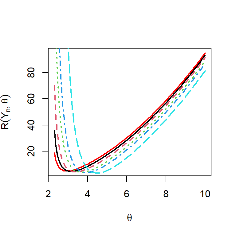
Let us check how the shapes changes with respect to sample size \(n\). The most important observation from Figure 6.14 is that as \(n\to \infty\), \(\mathcal{R}(Y_n,\theta) \not\to 0\), therefore \(Y_n\) is not a mean squared consistent estimator, which is certainly not a desirable property. The example of \(Y_n\) is just for an illustration purpose, how for a given statistic what properties to look at. In the following, we compare two estimators of \(\theta\), one is the method of moment and the other one is the MLE.
n_vals =c(10,20,50,100,500)n =5par(mfrow =c(1,1))curve(risk_fun_Yn(x), 2.3, 10, col ="red", lwd =2, ylab =expression(R(Y[n],theta)), xlab =expression(theta))for(i in1:length(n_vals)){ n = n_vals[i]curve(risk_fun_Yn(x), col = i, lwd =2, lty = i, add =TRUE)}
Figure 6.14: The risk function of the maximum order statistics for different choices of the sample size \(n\) under the squared error loss.
6.8.1 Method of moments Estimator
Using the method of moments, we can obtain an estimate of \(\theta\). The population mean \(\mbox{E}(X) = \frac{1}{\theta-1}\), which exists only when \(\theta\in(1,\infty)\). Therefore, equating the sample mean \(\overline{X_n}\) with population mean, we obtain the method of moment estimator of \(\theta\) as \[\widehat{\theta_{\mbox{MOM}}} = \frac{1}{\overline{X_n}+1} = V_n (\mbox{say})\]
6.8.2 Method of Maximum Likelihood
Using the method of maximum likelihood, we can also obtain the estimator of \(\theta\) as follows: The likelihood function is given by \[\mathcal{L}(\theta) = \prod_{i=1}^n \frac{\theta}{(1+x_i)^{1+\theta}}, 0<\theta<\infty\] and the log-likelihood function is given by \[l(\theta) = n \log \theta - n \sum_{i=1}^n \log(1+x_i).\] Equating \(l'(\theta) = 0\) implies, \(\theta^* = \frac{n}{\sum_{i=1}^n \log(1+x_i)}\) and \(l''(\theta) = -\frac{n}{\theta^2}<0\) for all \(\theta\in (0,\infty)\). Therefore, \(l(\theta)\) attains its maximum at \(\theta^*\). Therefore, the Maximum Likelihood Estimator of \(\theta\) is given by \[\widehat{\theta_{\mbox{MLE}}} = \frac{n}{\sum_{i=1}^n \log\left(1+X_i\right)} = W_n ~~(\mbox{say}).\]
As per our notation, \(V_n\) and \(W_n\) are the method of moments and maximum likelihood estimators of \(\theta\), respectively. Now we have three estimators of \(\theta\) and we are interested in comparing their risk functions which are listed as \(\mathcal{R}(Y_n,\theta)\), \(\mathcal{R}(V_n,\theta)\) and \(\mathcal{R}(W_n,\theta)\). It is important to note that the risk functions may exists only on a subset of the parameter space \(\Theta = (0,\infty)\).
We first try to compute the sampling distribution of \(W_n\). We compute it step by step.
Consider \(Y = \log(1+X)\), then the CDF of \(Y\) is given by \[\begin{eqnarray}
F_Y(y) = \mbox{P}(Y\le y) &=& \mbox{P}(\log(1+X)\le y) \\
&=& \mbox{P}\left(X\le e^y-1\right)\\
&=& 1-e^{-\theta y}, 0<y<\infty.
\end{eqnarray}\]
Therefore, \(Y=\log(1+X) \sim \mbox{Exponential}(\mbox{rate}=\theta)\) which is \(\mathcal{G}\left(\alpha = 1, \beta = \frac{1}{\theta}\right)\) distribution.
Let \(Y_i = \log\left(1+X_i\right), 1\le i\le n\), then by using the Moment Generating Function technique, we can easily show that \(Z_n=\sum_{i=1}^n Y_i = \sum_{i=1}^n \log(1+X_i)\sim \mathcal{G}(\alpha =n, \beta = \frac{1}{\theta})\), whose PDF is given by \[f_{Z_n}(z) = \frac{\theta^n z^{n-1}e^{-\theta z}}{\Gamma(n)}, 0<z<\infty.\] and zero otherwise.
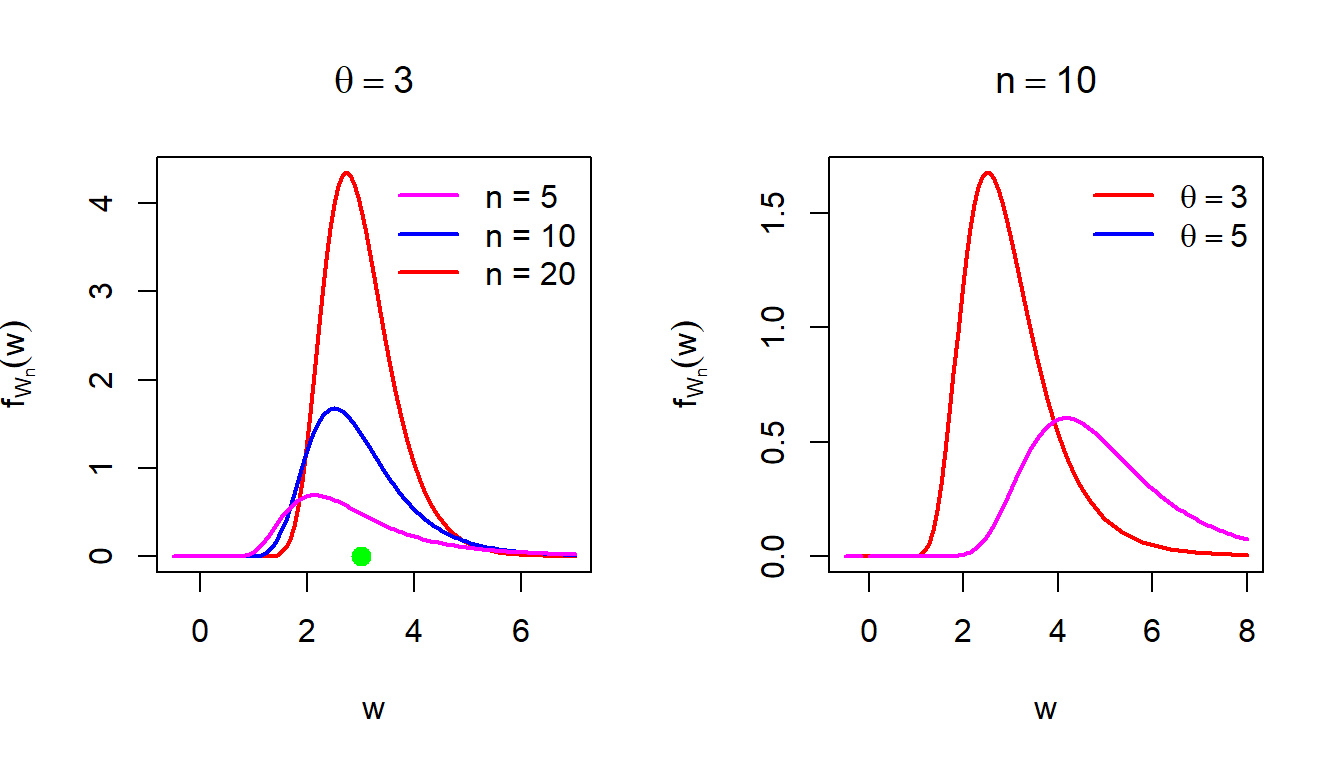
The MLE \(W_n = \frac{n}{Z_n}\). Using the transformation formula, we obtain \(f_{W_n}(w)\) as \[f_{W_n}(w) = f_{Z_n}\left(\frac{n}{w}\right)\left|\frac{d}{dw}\left(\frac{n}{w}\right)\right|, 0<w<\infty,\] which gives the PDF of \(W_n\) as \[f_{W_n}(w) = \frac{n (n\theta)^n e^{-\frac{n\theta}{w}}}{w^{n+2} \Gamma(n)}, 0<w<\infty,\] and zero otherwise. In the following R code, we visualize the sampling distribution of the MLE of \(\theta\) (PDF) for different choices of \(\theta\) and sample size \(n\).
Figure 6.15: The sampling distribution of the MLE \(W_n\) of \(\theta\) for different choices of \(\theta\) and different sample size. Left panel: As the sample size increases, the sampling distribution of \(W_n\) is highly concentrated about the true value of \(\theta = 3\), which is a desirable property of the MLE (consistency).
To compute the risk \(\mathcal{R}(W_n,\theta)\), we compute
Therefore, the risk under the squared error loss is given by \[\begin{eqnarray}
\mbox{E}_{\theta}\left(W_n -\theta\right)^2 &=& \mbox{E}_{\theta}(W_n^2)-2\theta \mbox{E}_{\theta}(W_n) + \theta^2 \\
&=& \frac{\theta^2(n+2)}{(n-1)(n-2)}, n>2.
\end{eqnarray}\] The following observation is important.
\(\mbox{Bias}_{\theta}(W_n) = \mbox{E}_{\theta}(W_n)-\theta = \frac{n\theta}{n-1}-\theta = \frac{\theta}{n-1}\to 0\) as \(n\to \infty\). Therefore, \(W_n\) is asymptotically unbiased estimator.
\(\mathcal{R}(W_n,\theta) = \mbox{E}_{\theta}(W_n-\theta)^2\to 0\) as \(n\to \infty\). Therefore, \(W_n\to \theta\) in probability as \(n\to \infty\) (a simple application of Markov Inequality).
Let us now verify whether the theoretical computation of the risk function for the \(W_n\) is supported by the simulation study as well. We follow the same scheme as previous.
Fix \(\theta\) and fix \(n\), sample size.
Simulate \(X_1,X_2,\ldots,X_n \sim f(x|\theta)\)
Compute \(W_n\)
Compute the loss \((W_n-\theta)^2\)
Repeat the above three steps \(M\) times to compute the average loss.
Repeat above five steps for different choices of \(\theta\) from the parameter space.
Plot the average loss values (approximate risk) at each value of \(\theta\).
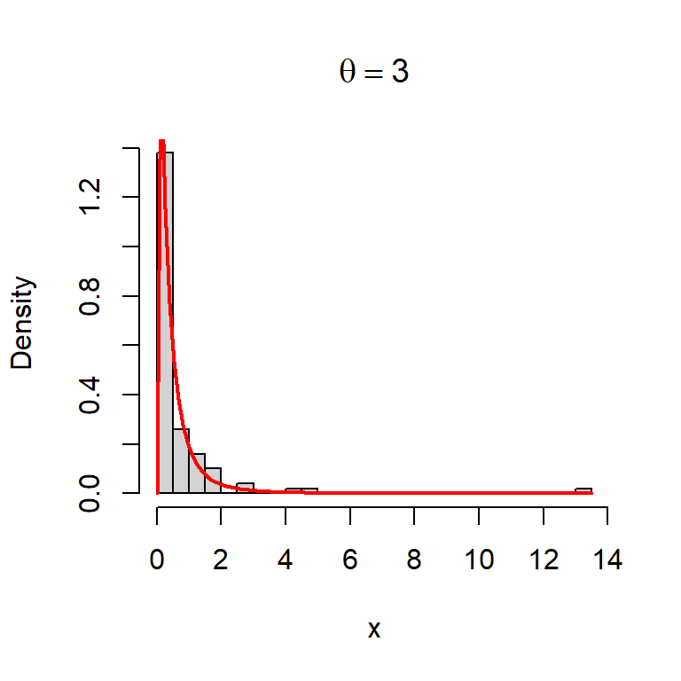
In the above algorithm, primary challenge is to simulate from the given PDF as some inbuilt function may not be available to directly simulate using R or Python. Let us use the probability integral transform to simulate \(X_1,\ldots,X_n\sim f(x|\theta)\). Simulate \(U\sim \mbox{Uniform}(0,1)\) and compute \(X = F_X^{-1}(U)\), where \(F_X^{-1}\) is the inverse of the CDF. In this case, the equation to generate \(X\sim f(x|\theta)\) becomes \[X = (1-U)^{-\frac{1}{\theta}} - 1, 0<U<1.\] In the following first verify whether the simulation study.
n =100theta =3# true parameter valueu =runif(n = n, min =0, max =1) # simulate U(0,1)x = (1-u)^(-1/theta) -1# probability integral transformhist(x, probability =TRUE, main =bquote(theta == .(theta)),breaks =30) # histogramcurve(f(x), add =TRUE, col ="red", lwd =2) # add the original pdf
Figure 6.16: simulated realization from the given PDF \(f(x;\theta=3)\) using probability integral transform.
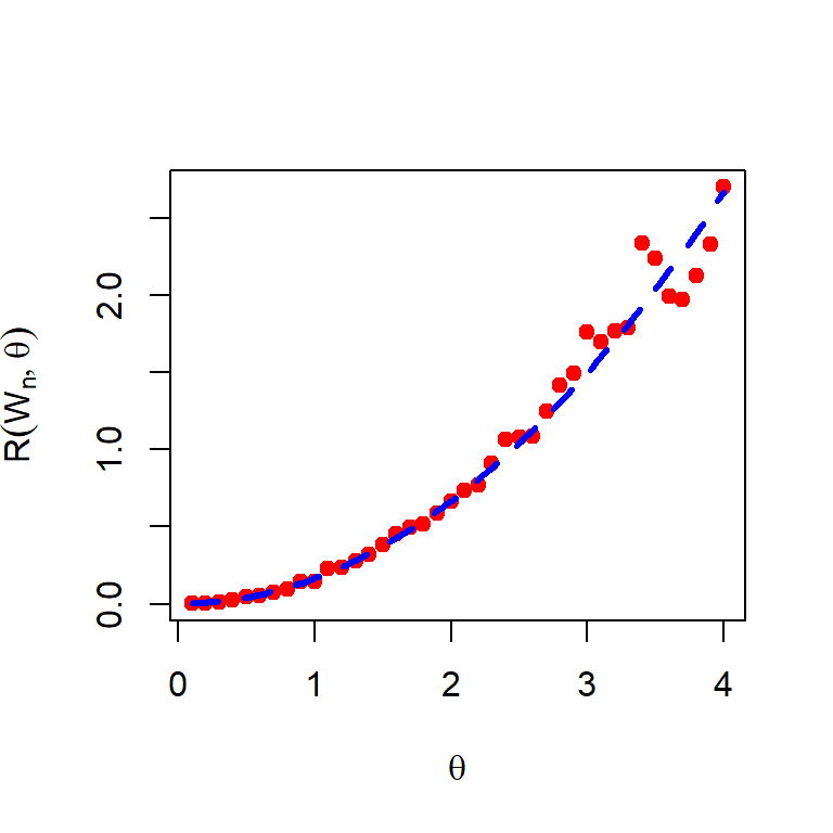
Let us now execute simulation of the risk function using computer simulation and verify with the theoretical result.
M =1000# number of replicationsn =10theta_vals =seq(0.1, 4, by =0.1)risk_vals =numeric(length =length(theta_vals))for(i in1:length(theta_vals)){ theta = theta_vals[i] loss_vals =numeric(length = M)for(j in1:M){ u =runif(n = n, min =0, max =1) x = (1-u)^(-1/theta) -1 W_n = n/sum(log(1+x)) loss_vals[j] = (W_n - theta)^2 } risk_vals[i] =mean(loss_vals)}plot(theta_vals, risk_vals, col ="red", pch =19, xlab =expression(theta), ylab =expression(R(W[n],theta)))curve(x^2*(n+2)/((n-1)*(n-2)), lwd =3, col ="blue",add =TRUE, lty =2)
Figure 6.17: The risk function is obtained by computer simulation for the MLE \(W_n\) of \(\theta\). True risk function is added for reference (blue dotted line).
The MLE \(W_n\) has desirable properties. We are yet to check it for the Method of Moment estimator \(V_n\).
6.8.3 Approximation of \(\mathcal{R}(V_n,\theta)\)
The exact sampling distribution of the method of moment estimator \(V_n = \overline{X_n}^{-1}+1\) is difficult to obtain. Therefore, an analytically tractable expression of the risk function is almost impossible to obtain. However, we can possibly obtain an approximation of the risk function for large sample size \(n\) for a subset of the parameter space \(\Theta = (0,\infty)\). In the following, we first obtain the risk function by computer simulation.
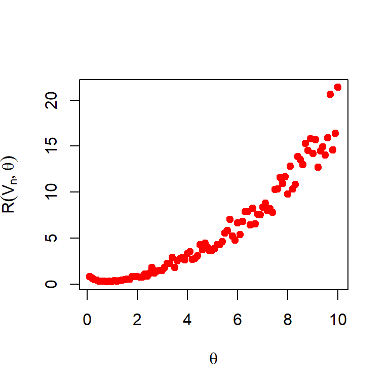
M =500# number of replicationsn =10# sample sizetheta_vals =seq(0.1, 10, by =0.1) # different theta valuesrisk_vals =numeric(length =length(theta_vals))for(i in1:length(theta_vals)){ theta = theta_vals[i] loss_vals =numeric(length = M)for(j in1:M){ u =runif(n = n, min =0, max =1) x = (1-u)^(-1/theta) -1 V_n =1/mean(x)+1 loss_vals[j] = (V_n - theta)^2 } risk_vals[i] =mean(loss_vals)}plot(theta_vals, risk_vals, col ="red", pch =19, xlab =expression(theta), ylab =expression(R(V[n],theta)))
Figure 6.18: The risk function is obtained by computer simulation for the MLE \(W_n\) of \(\theta\).
\(\mbox{E}(X) = \mu = \frac{1}{\theta - 1}\) exists for \(\theta>1\) and \(Var(X)= \sigma^2= \frac{2}{(\theta - 1)(\theta -2)}\) which exists for \(\theta\in (2,\infty)\). Therefore, when \(\theta\in(2,\infty)\), we can apply the CLT, which ensures the large sample approximation of the sampling distribution of \(\overline{X_n}\) as \[\overline{X_n} \sim \mathcal{N}\left(\frac{1}{\theta-1}, \frac{2}{n(\theta-1)(\theta-2)}\right).\] Now we can approximate the sampling distribution of \(g(\overline{X_n}) = \overline{X_n}^{-1}+1\) by using first order Taylor’s approximation and \(g(\mu) = \frac{1}{\mu}+1 = \theta\).
\[g\left(\overline{X_n}\right)\approx g(\mu) + \left(\overline{X_n}-\mu\right)g'(\mu)\] which implies
\[V_n = \frac{1}{\overline{X_n}}+1 \approx \frac{1}{\mu} + 1 +\left(\overline{X_n} - \mu\right)\left(-\frac{1}{\mu^2}\right)=\theta+\left(\overline{X_n} - \frac{1}{\theta-1}\right)\left(-(\theta-1)^2\right)\] Therefore, by the first order Taylor Approximation, \[\mbox{E}_{\theta} (V_n) \approx \theta\] and the variance is obtained as \[\begin{eqnarray}
Var_{\theta}(V_n) &\approx& \mbox{E}_{\theta}\left(V_n-\theta\right)^2\\
& =& \mbox{E}_{\theta}\left(\overline{X_n} - \frac{1}{\theta-1}\right)^2 (\theta-1)^4\\
&=& Var_{\theta}\left(X_n\right)(\theta-1)^2\\
&\approx & \frac{1}{n(\theta-1)(\theta-2)}(\theta-1)^4 = \frac{(\theta-1)^3}{n(\theta-2)}.\end{eqnarray}\] Therefore, by the application of Delta method \[V_n = g\left(\overline{X_n}\right)\sim \mathcal{N}\left(\theta, \frac{(\theta-1)^3}{n(\theta-2)}\right), \mbox{for large }n, \theta\in(2,\infty)\] In the following code, the above approximation is verified by computer simulation.
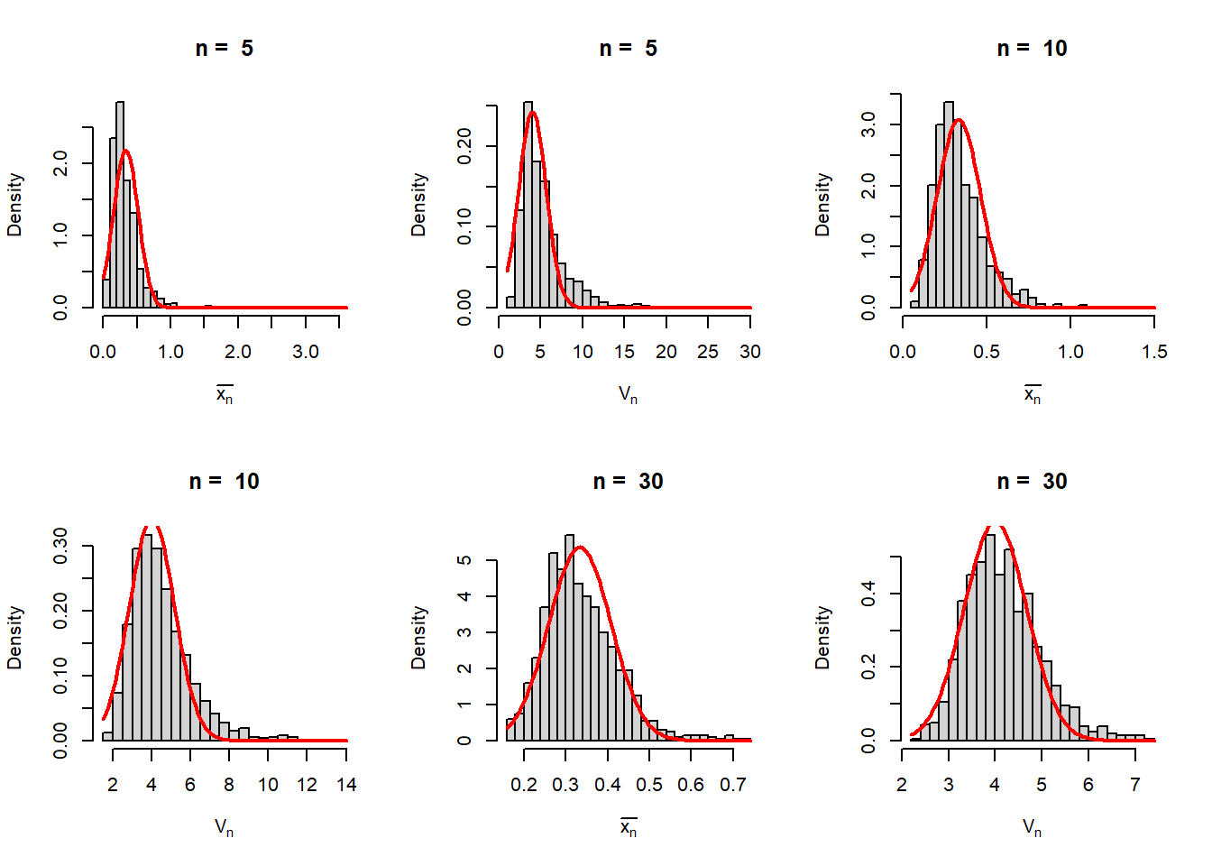
M =1000theta =4# true value of thetan_vals =c(5, 10, 30, 50, 100,500)par(mfrow =c(2,3))for(n in n_vals){ xbar =numeric(length = M) g_xbar =numeric(length = M)for(i in1:M){ u =runif(n = n, min =0, max =1) x = (1-u)^(-1/theta) -1# probability integral transform xbar[i] =mean(x) g_xbar[i] =1/mean(x) +1 }hist(xbar, probability =TRUE, main =paste("n = ", n),xlab =expression(bar(x[n])), breaks =30)curve(dnorm(x, mean =1/(theta-1), sd =sqrt(1/(n*(theta-1)*(theta-2)))), col ="red", lwd =2, add =TRUE)hist(g_xbar, probability =TRUE, main =paste("n = ", n),xlab =expression(V[n]), breaks =30)curve(dnorm(x, mean = theta, sd =sqrt((theta-1)^3/(n*(theta-2)))),col ="red", lwd =2, add =TRUE)}
Figure 6.19: As the sample size increases, the sample mean \(\overline{X_n}\) is approximately normally distributed with mean \(\mu = \frac{1}{\theta - 1}\) and variance \(\frac{\sigma^2}{n}=\frac{1}{n(\theta-1)(\theta-2)}\). Using the first order Taylor’s approximation the sampling distribution of \(V_n\) is obtained by computer simulation. The sampling distribution is well approximated by the normal distribution for large \(n\). The approximate mean and variance of \(V_n\) is provided in the main text.
Figure 6.20: As the sample size increases, the sample mean \(\overline{X_n}\) is approximately normally distributed with mean \(\mu = \frac{1}{\theta - 1}\) and variance \(\frac{\sigma^2}{n}=\frac{1}{n(\theta-1)(\theta-2)}\). Using the first order Taylor’s approximation the sampling distribution of \(V_n\) is obtained by computer simulation. The sampling distribution is well approximated by the normal distribution for large \(n\). The approximate mean and variance of \(V_n\) is provided in the main text.
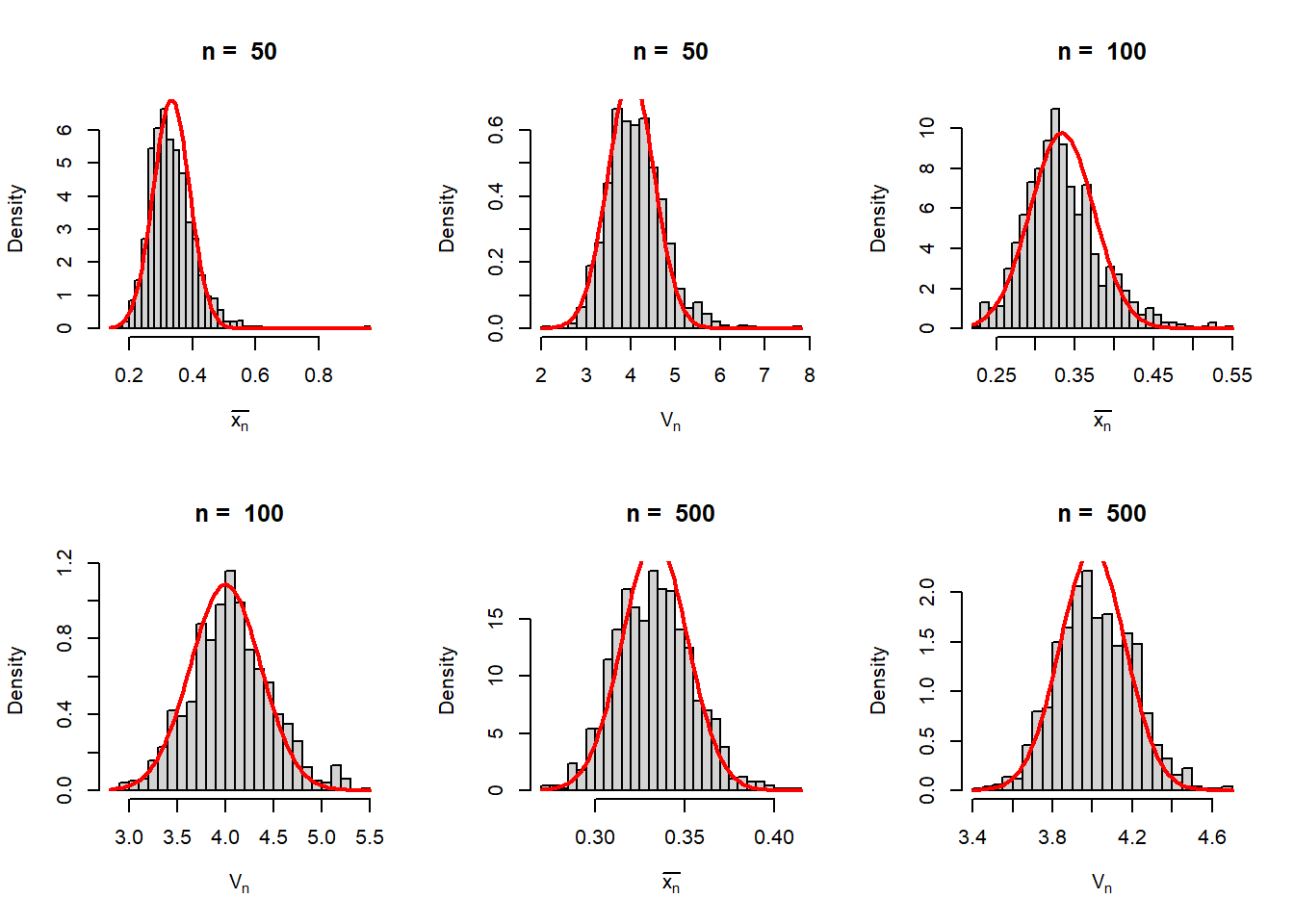
n_vals =c(5, 10, 25, 50, 100, 500)theta_vals =seq(3, 20, by =0.5)par(mfrow =c(2,3))M =500# number of replicationsfor(n in n_vals){ risk_vals =numeric(length =length(theta_vals))for(i in1:length(theta_vals)){ theta = theta_vals[i] loss_vals =numeric(length = M)for(j in1:M){ u =runif(n = n, min =0, max =1) x = (1-u)^(-1/theta) -1 V_n =1/mean(x)+1 loss_vals[j] = (V_n - theta)^2 } risk_vals[i] =mean(loss_vals) }plot(theta_vals, risk_vals, col ="red", pch =19, xlab =expression(theta), ylab =expression(R(V[n],theta)),main =paste("n = ", n))curve((x-1)^3/(n*(x-2)), add =TRUE, col ="blue", lty =2,lwd =2)}
Figure 6.21: The approximation of the risk function of \(V_n\) by the first order Taylor’s approximation. As \(n\to \infty\), the approximations are accurate.
6.8.4 Comparing estimators \(V_n\) and \(W_n\)
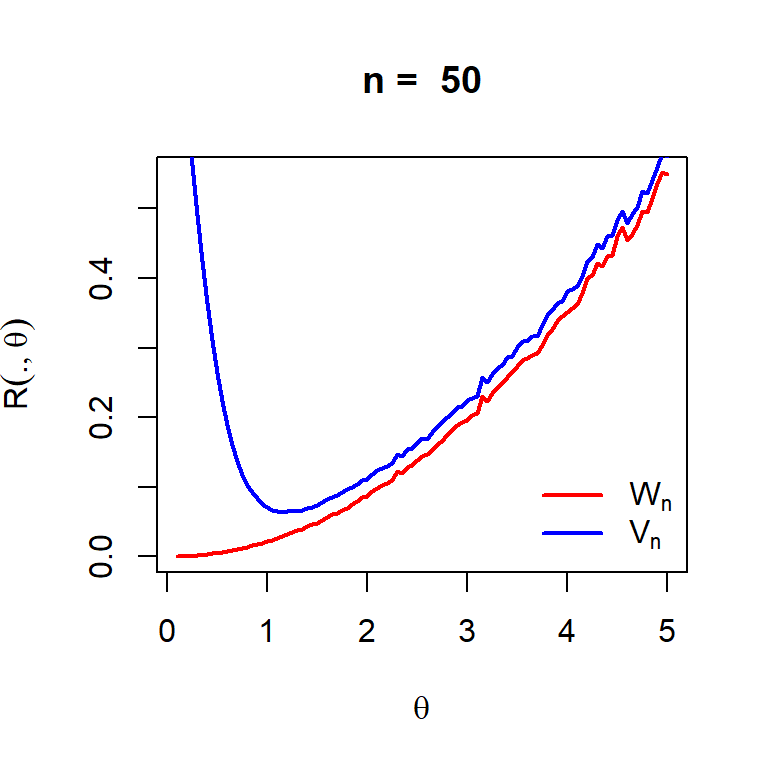
n =50theta_vals =seq(0.1,5, by =0.05)M =10000risk_Vn =numeric(length =length(theta_vals)) # method of momentsrisk_Wn =numeric(length =length(theta_vals)) # method of maximum likelihoodfor (i in1:length(theta_vals)) { theta = theta_vals[i] loss_Vn =numeric(length = M) loss_Wn =numeric(length = M)for(j in1:M){ u =runif(n = n, min =0, max =1) x = (1-u)^(-1/theta) -1 V_n =1/mean(x) +1 W_n = n/sum(log(1+x)) loss_Vn[j] = (V_n - theta)^2 loss_Wn[j] = (W_n - theta)^2 } risk_Vn[i] =mean(loss_Vn) risk_Wn[i] =mean(loss_Wn)}plot(theta_vals, risk_Wn, col ="red", lwd =2, type ="l",xlab =expression(theta), ylab =expression(R(., theta)),main =paste("n = ", n))lines(theta_vals, risk_Vn, col ="blue", lwd =2)legend("bottomright", legend =c(expression(W[n]), expression(V[n])), col =c("red", "blue"),lwd =c(2,2), bty ="n")
Figure 6.22: Comparison of the risk function of the method of moments and method of maximum likelihood. It can be observed that the MLE has uniformly smaller risk than the MoM estimator. Therefore, \(W_n\) is a preferred estimator than \(V_n\). Similar exercise can be carried out for \(Y_n\) as well and we can find that MLE has outperformed both the estimator. A natural question arises, is MLE the best among all estimators of \(\theta\). This will be answered in the next chapter.