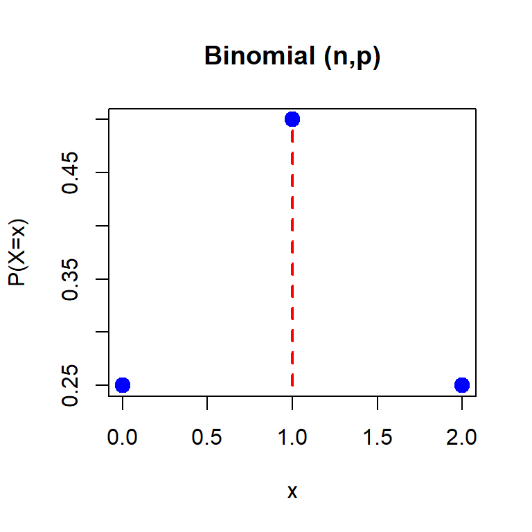
Suppose that we have a fair coin and we toss it two times, then the sample space is given by \[\mathcal{S} = \{HH, TH, HT, TT\}\] Suppose that \(X\colon \mathcal{S}\to \mathbb{R}\), defined as \[X(s) = \mbox{number of H in }s,\] therefore \(X\in \{0,1,2\}\). Since it is a fair coin, the following probabilities can be easily computed. \[\mbox{P}(X=0) = \frac{1}{4},~~\mbox{P}(X=1) = \frac{1}{2}, ~~\mbox{P}(X=2) = \frac{1}{4}.\] We can visualize these values as a mass on the real line having masses at the values \(\{0,1,2\}\). Let us visualize it using R.
In the following, we first visualize the probability mass function for \(n=2\).
n =2# number of throwsx =0:n # possible values of the random variable Xprint(x)
[1] 0 1 2
p =0.5# probability of headp_x =choose(n, x)*p^x*(1-p)^(n-x)print(p_x)
Figure 4.1: The probability mass function of the binomial probability distribution when the coin is fair. The random variable \(X\) represents the number of heads when the coin is tossed twice.
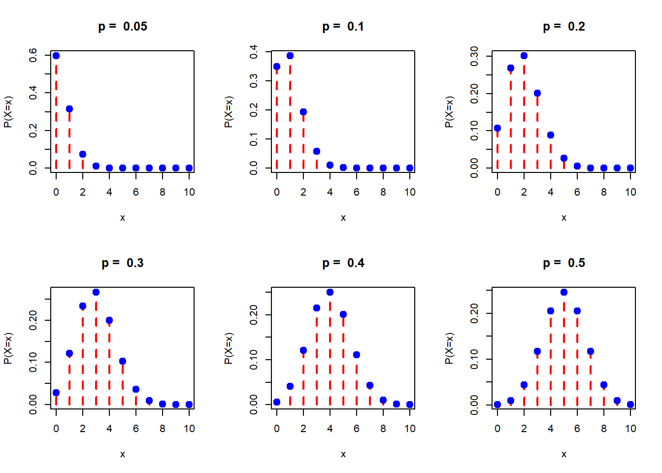
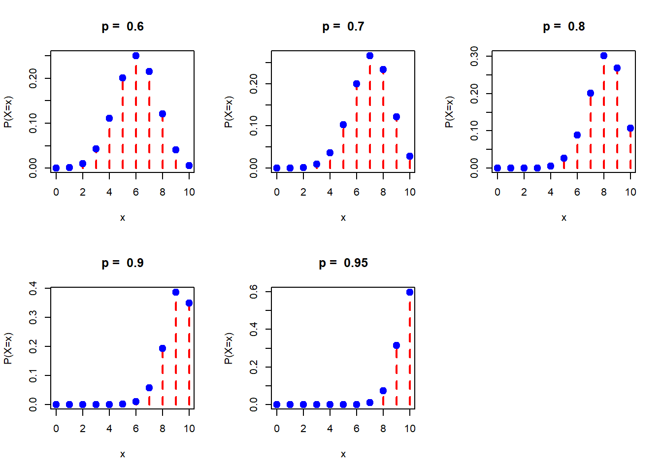
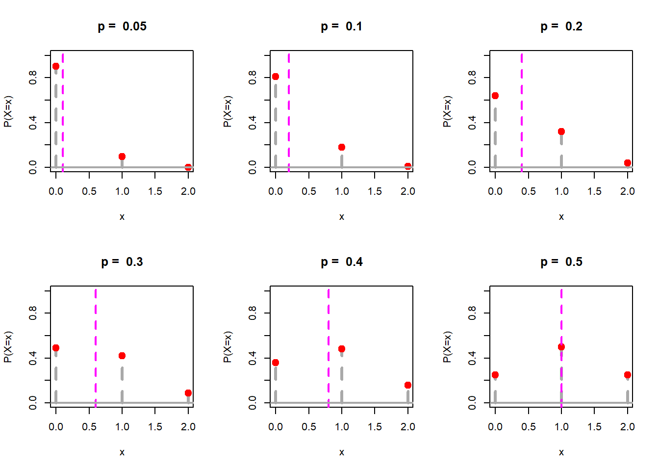
For \(n = 10\), we now visualize various shapes of PMF of \(X\) for different choice of \(p\in(0,1)\). We can now generalize this situation to consider a coin with probability of head as \(p\in(0,1)\). Therefore, we are considering tossing with a biased coin as well. It is easy to compute that (based on the classroom exercise) is that
\[\mbox{P}(X=x) = {2\choose{x}} p^x(1-p)^{2-x}, x\in\{0,1,2\},\] and zero otherwise. In the following, we check various shapes of the distribution of the mass on the real line.
Listing 4.1: R Code: The reader is encouraged to see how the loop is written for different choices of \(p\).
p_vals =c(0.05, seq(0.1, 0.9, by =0.1), 0.95) # different values of prob of head print(p_vals)n =10par(mfrow =c(2,3))for (p in p_vals) { x =0:n p_x =choose(n, x)*p^x*(1-p)^(n-x)print(p_x)plot(x, p_x, pch =19, ylab ="P(X=x)", type="h", lwd =2,col ="red", lty =2, main =paste("p = ", p))points(x, p_x, pch =19, col ="blue", cex =1.5)}
Figure 4.2: The shapes of the binomial PMF for different choice of the success probability \(p\). As \(p\) is close to 1, more number of heads is expected to occur.
Figure 4.3: The shapes of the binomial PMF for different choice of the success probability \(p\). As \(p\) is close to 1, more number of heads is expected to occur.
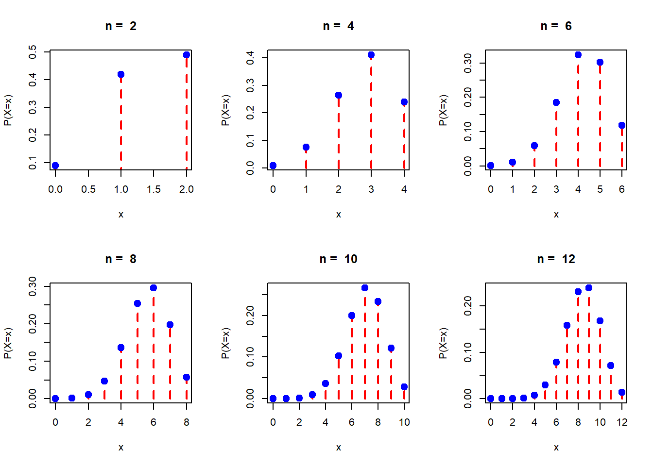
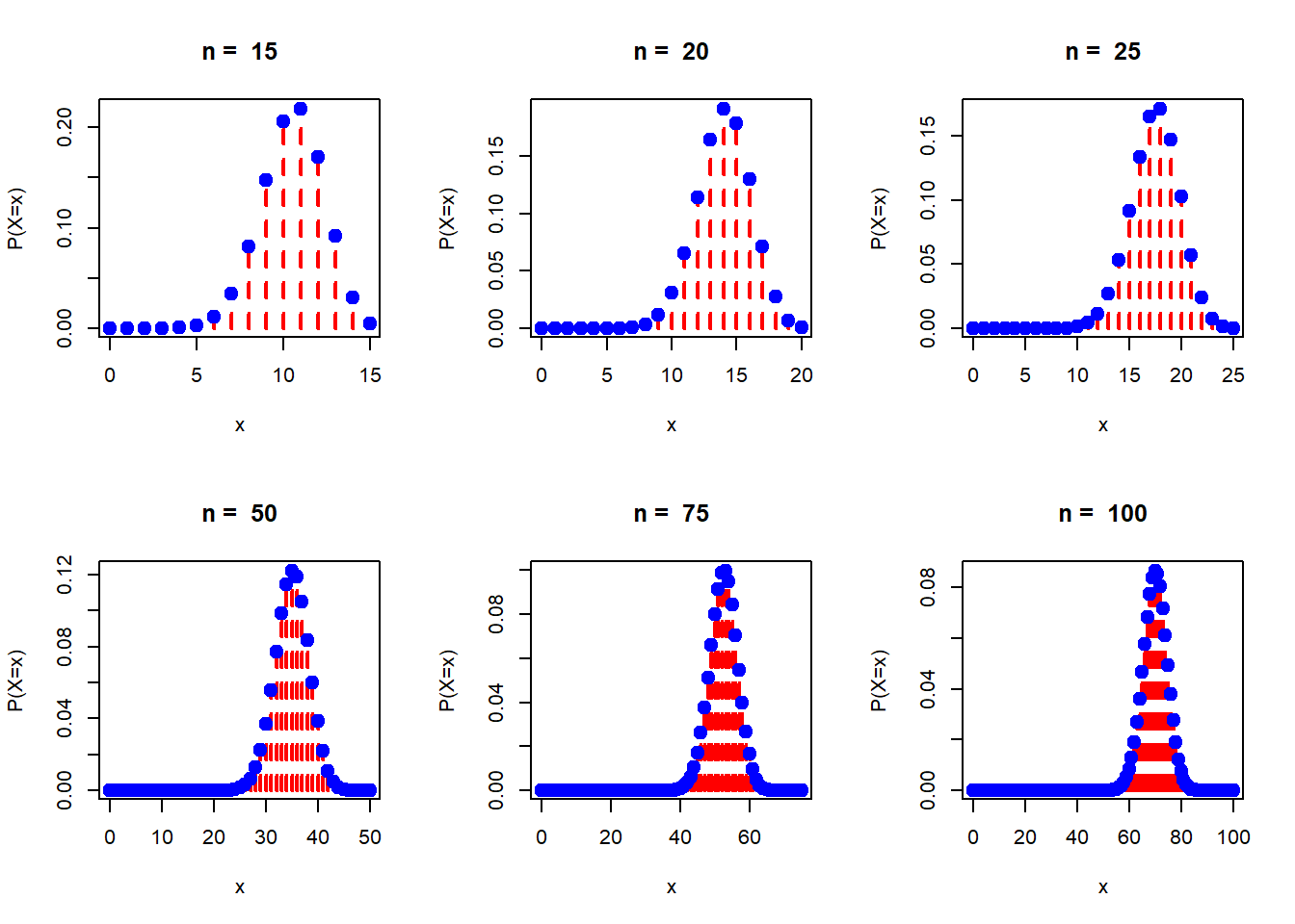
Listing 4.2: R Code: The reader is encouraged to see how the loop is written for different choices of \(n\).
Figure 4.4: The shapes of the binomial PMF for different choice of \(n\) and the success probability \(p\) is fixed.
Figure 4.5: The shapes of the binomial PMF for different choice of \(n\) and the success probability \(p\) is fixed.
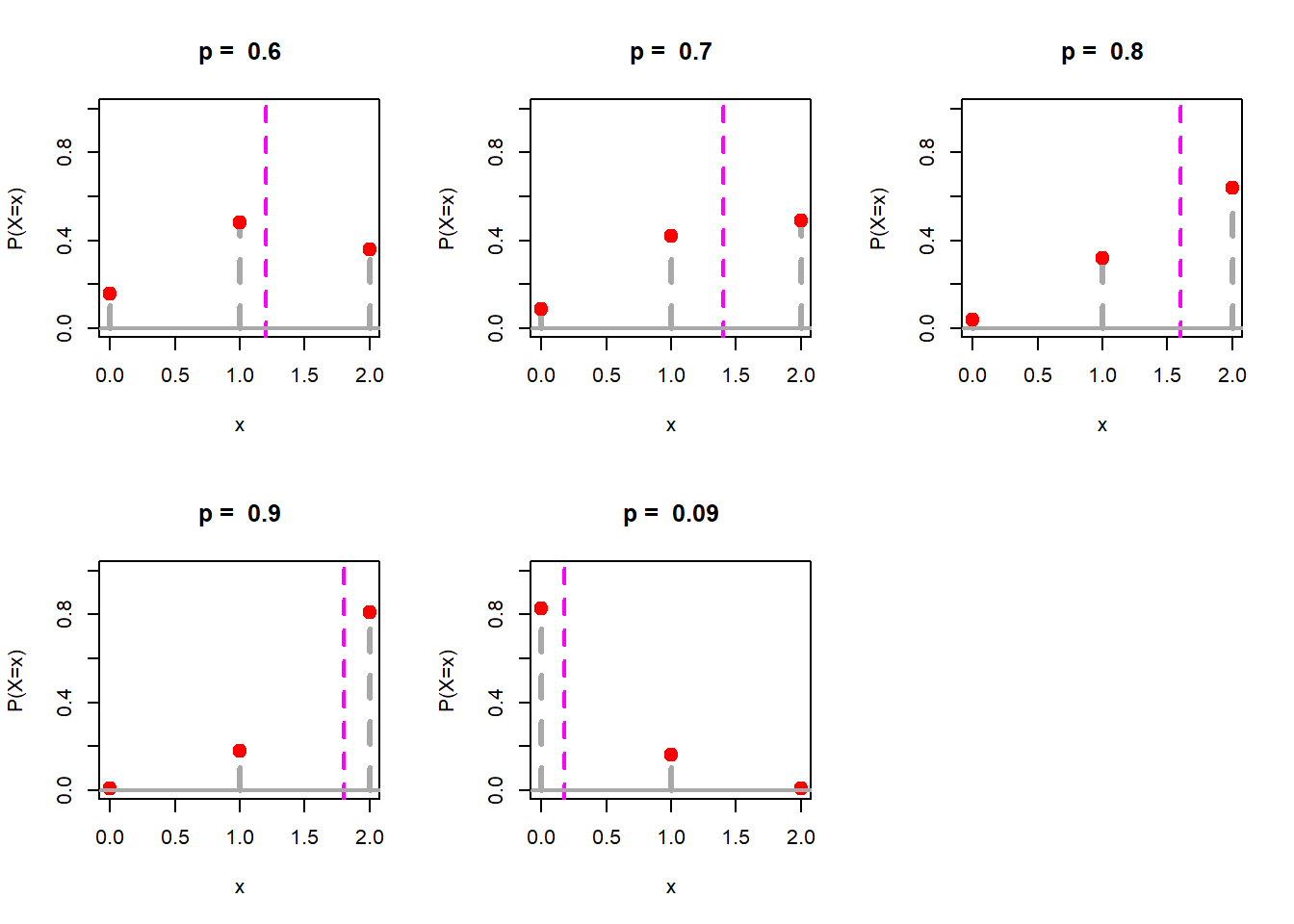
We can compute the center of mass of these masses using the formula \(\sum m_ix_i/\sum m_i\). You can check that the center of mass is given by \(2p\). It can be easily verified that if the coin is tossed thrice, then the center of mass is given by \(3p\). In the plot, we have added the centre of mass using a vertical magenta colored dotted line.
Listing 4.3: R Code: The students are encouraged to realize that how simple plots can be more effective for a better understanding of the concepts. We usually compute the expectation in a mathematical way and hardly realize its use. However, the idea of center of mass or the average value give a better understanding of the concepts.
n =2# number of throwsp_vals =c(0.05, seq(0.1, 0.9, by =0.1), 0.09)par(mfrow =c(2,3))x =0:n # values taken by Xfor(p in p_vals){ p_x =choose(n, x)*p^x*(1-p)^(n-x) # probability valuesplot(x, p_x, pch =19, type ="h", ylab ="P(X=x)",cex =1.3, col ="darkgrey", ylim =c(0,1),lwd =3, main =paste("p = ", p), lty =2)points(x, p_x, pch =19, col ="red",cex =1.5) CM = n*p # expected valueabline(v = CM, col ="magenta",lwd=2, lty =2)abline(h =0, col ="darkgrey", lwd =2) }
Figure 4.6: It should be noted that as the probability of head changes, the center of mass (the expected value) also changes. For example, as \(p\) increases, the mass shifts towards the right. When \(p=\frac{1}{2}\), the center of mass is exactly at the point 1. The vertical dotted magenta color line indicates the center of mass. For students, it may be considered that the point through which the eartch is attracting the mass.
Figure 4.7: It should be noted that as the probability of head changes, the center of mass (the expected value) also changes. For example, as \(p\) increases, the mass shifts towards the right. When \(p=\frac{1}{2}\), the center of mass is exactly at the point 1. The vertical dotted magenta color line indicates the center of mass. For students, it may be considered that the point through which the eartch is attracting the mass.
Classroom exercises
Find the value of \(a\) so that the following function is a PMF. \[g(x) = \begin{cases} a\frac{\lambda^x}{x!},~x\in\{0,1,2,\ldots,\} \\ 0,~~~~\mbox{otherwise} \end{cases}.\] Plot the PMF for \(\lambda \in \{1,2,3,4,5,6\}\). Use the option \(\texttt{par(mfrow = c(2,3))}\)
Find the value of \(a\) so that the following function is a PMF: \[g(x) = \begin{cases} \frac{a}{x^2},~x\in\{0,1,2,\ldots,100\} \\ 0,~~~~\mbox{otherwise} \end{cases}.\]
Find the value of \(a\) so that the following function is a PMF: \[g(x) = \begin{cases} a(1-p)^{x-1},~x\in\{1,2,\ldots\} \\ 0,~~~~\mbox{otherwise} \end{cases}.\] Plot the PMF using R for different choices of \(p\).
Find the value of \(a\) so that the following function is a PMF: \[g(x) = \begin{cases} \frac{a}{n+1},~x\in\{0,1,2,\ldots,n\}, \mbox{ where } n\in \mathbb{N} \\ 0,~~~~\mbox{otherwise} \end{cases}.\]
4.1 Probability density function
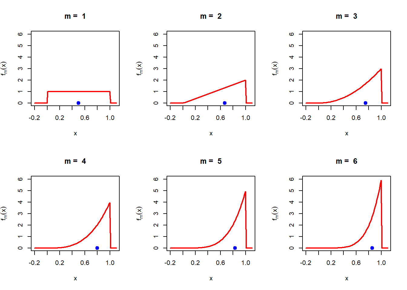
In the above discussion, we have considered random variable that takes only a finite or countable values on the real line. We start our discussion with a family of functions \(f_m(x)\), \(m\in\{1,2,3,\ldots\}\), which is defined as \[f_m(x) = \begin{cases} mx^{m-1},~~0<x<1, \\ 0,~~~~~~~~~~~~\mbox{Otherwise}. \end{cases} \tag{4.1}\] In the following, we first draw a shape of these functions using the following code
Listing 4.4: R Code: The students are encouraged to see how the support of the probability density function is given in the body of the function using the star symbol
f_m =function(x){ m*x^(m-1)*(x>0)*(x<1)}par(mfrow =c(2,3))m_vals =1:6# different values of mfor(m in m_vals){curve(f_m(x), col ="red", lwd =2, main =paste("m = ", m),xlim =c(-0.2, 1.1), ylim =c (0,6), ylab =expression(f[m](x)))points(m/(m+1), 0, pch =19, col ="blue", cex =1.3)}
Figure 4.8: The shape of the function \(f_m(x)\) for different choices of \(m\).
Probability density function
A function \(f(x)\) is called a probability density function (PDF) if
\(f(x)\ge 0\) for all \(x\in (-\infty, \infty)\).
\(\int_{-\infty}^{\infty} f(x)dx = 1\).
Using the \(\texttt{integrate()}\) function, we can check whether the functions \(f_m(x), m\in\{1,2,3,\ldots,\}\) are PDF or not. Before doing it by using R, we can easily check that by using the direct integration as follows: \[\begin{aligned} \int_{-\infty}^{\infty} f_m(x)dx &= \int_{-\infty}^0f_m(x)dx + \int_0^1 f_m(x)dx+ \int_{1}^{\infty}f_m(x)dx \\
&=\int_{-\infty}^00\cdot dx + \int_0^1 mx^{m-1}dx+ \int_{1}^{\infty}0\cdot \\ &= m \left[\frac{x^m}{m}\right]_{x=0}^{x=1} = 1.\end{aligned}\]
Using R, we can check whether the integral is 1.
m =3# change the value of mintegrate(f_m, lower =0, upper =1)
1 with absolute error < 1.1e-14
4.2 Some more examples
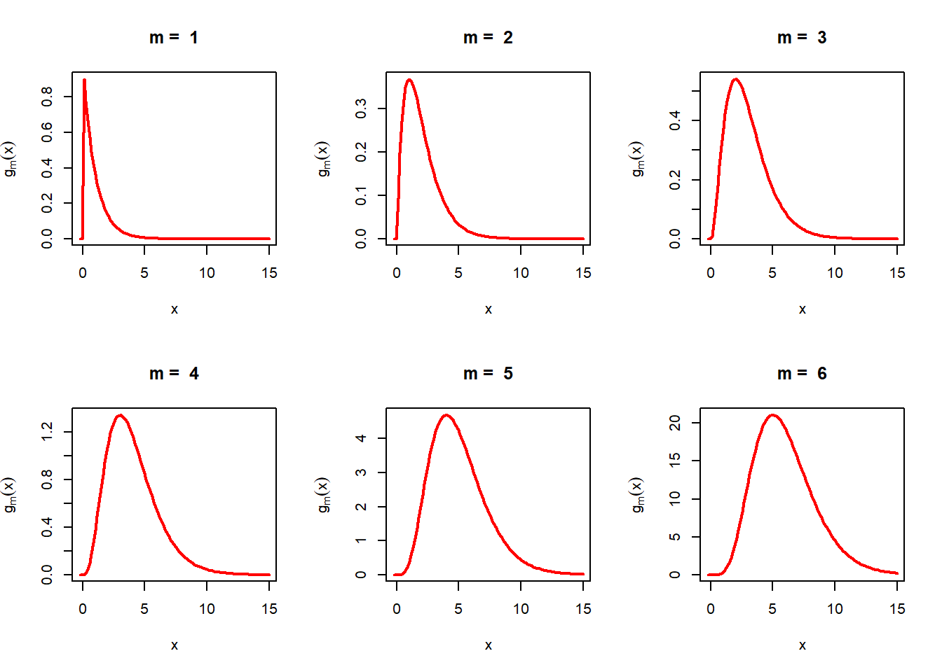
Suppose that we consider the set of functions \(g_m(x)\) for \(m\in\{1,2,\ldots,\}\)\[g_m(x) = \begin{cases} x^{m-1}e^{-x},~~0<x<\infty \\ 0, ~~~~~~~~~~~~~~\mbox{otherwise}.\end{cases}\]
In the classroom, many students may not be knowing about the \(\texttt{gamma()}\) function. In such a case, the instructor is encouraged to start with the computation of integration by hand \[\int_0^{\infty} g_m(x)dx, ~~\mbox{for}~~m\in\{1,2,3\}\] and come up with the generalization \[\int_0^{\infty} g_m(x)dx = (m-1)\int_0^{\infty}g_{m-1}(x)dx=\cdots =(m-1)!\] Let us now plot these functions
Listing 4.5: R Code: It is always a better option to plot the functions whichever is discussed during the lecture. This gives a better understanding for the students and the visual displays play a longstanding impact on the students. The students are encouraged to integrate these functions and see whether their theoretical computation matches with the output of the \(\texttt{integrate()}\) function.
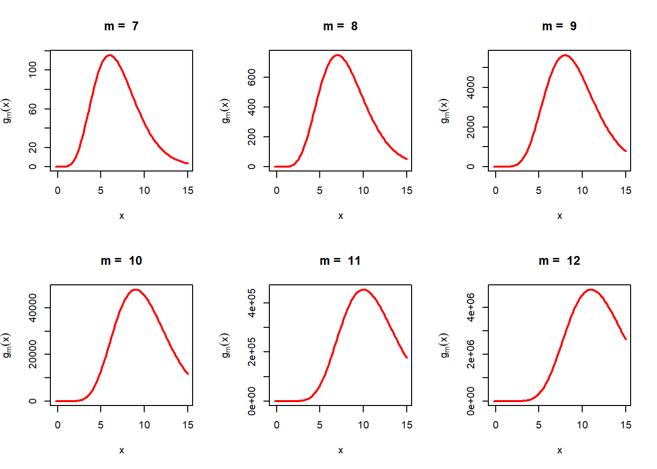
g_m =function(x){ x^(m-1)*exp(-x)*(x>0)}par(mfrow =c(2,3))m_vals =1:12for(m in m_vals){curve(g_m(x), col ="red", lwd =2, main =paste("m = ", m),xlim =c(-0.2, 15), ylab =expression(g[m](x)))}
Figure 4.9: The shape of the function \(g_m(x)\) for different choices of \(m\). It may be noted that close to zero \(x^m\) term dominates, and for large values of \(x\), the exponential term dominates and the PDF is exponentially decaying to zero as \(x\to \infty\).
Figure 4.10: The shape of the function \(g_m(x)\) for different choices of \(m\). It may be noted that close to zero \(x^m\) term dominates, and for large values of \(x\), the exponential term dominates and the PDF is exponentially decaying to zero as \(x\to \infty\).
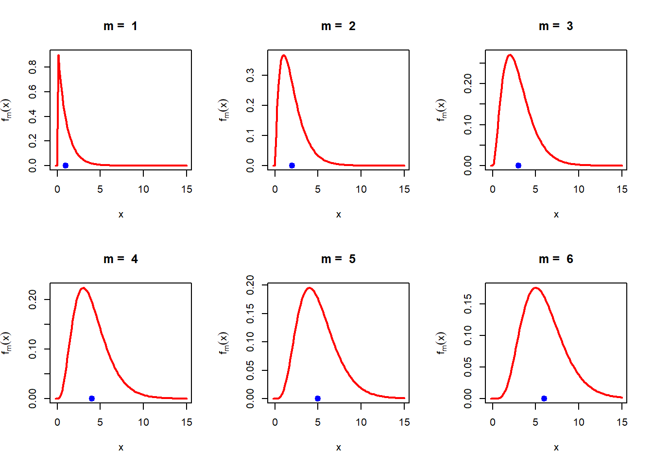
The following numerical integration output suggests that \(g_m(x)\) is PDF only for \(m=1\) and \(m=2\). However, for \(m\ge 3\), \(\int_0^{\infty}g_m(x)dx \ne 1\). However, these functions can be converted to the PDF by appropriately scaling them (by dividing with the total area under the curve) to probability density functions. Consider \[f_m(x) = \begin{cases} \frac{1}{(m-1)!}g_m(x),~ 0<x<\infty \\ 0,~~~~~~~~\mbox{Otherwise} \end{cases} = \begin{cases} \frac{e^{-x}x^{m-1}}{(m-1)!}, 0<x<\infty\\ 0,~~~~ \mbox{otherwise} \end{cases}.\]
for(m in m_vals){print(integrate(g_m, lower =0, upper =Inf))}
1 with absolute error < 5.7e-05
1 with absolute error < 6.4e-06
2 with absolute error < 7.1e-05
6 with absolute error < 2.6e-06
24 with absolute error < 2.2e-05
120 with absolute error < 7.3e-05
720 with absolute error < 0.0047
5040 with absolute error < 0.35
40320 with absolute error < 0.0013
362880 with absolute error < 0.025
3628800 with absolute error < 0.34
39916800 with absolute error < 3.1
Listing 4.6: R Code: It is important to note that we did not define the function again, rather we have passed the function \(g_m(x)\) to the body of the function \(f_m(x)\). Also note the use of the \(\texttt{factorial()}\) function.
par(mfrow =c(2,3))m_vals =1:6# different values of mf_m =function(x){g_m(x)/factorial(m-1)}for(m in m_vals){curve(f_m(x), col ="red",lwd =2, main =paste("m = ", m),xlim =c(-0.2, 15),ylab =expression(f[m](x)))points(m, 0, pch =19, col ="blue", cex =1.3)}
Figure 4.11: We first integrated the function \(g_m(x)\) and the obtain \(f_m(x)\) by dividing the total are under the function \(g_m(x)\). It should be noted that the integration is performed in the interval \((0,\infty)\) and the support of the distribution with the PDF \(f_m(x)\) is \((0,\infty)\).
Using the following R Code, we can verify that for different choices of \(m\), the area under the function \(f_m(x)\) is 1 in the interval \((0,\infty)\).
m_vals =1:6for(m in m_vals){print(integrate(f_m, lower =0, upper =Inf))}
1 with absolute error < 5.7e-05
1 with absolute error < 6.4e-06
1 with absolute error < 3.5e-05
1 with absolute error < 4.4e-07
1 with absolute error < 9.3e-07
1 with absolute error < 6.1e-07
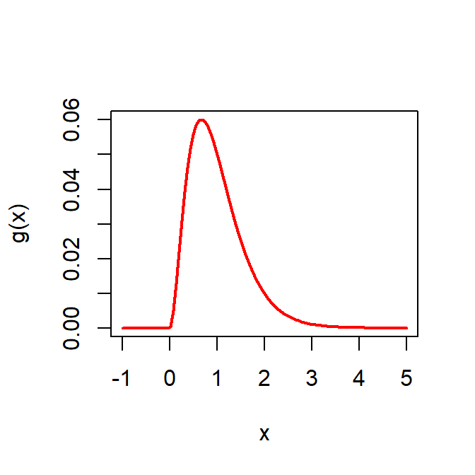
In the following, let us check whether the following function is a PDF. The function \[g(x) = x^2e^{-3x}, 0<x<\infty,\] and zero otherwise.
g =function(x){ x^2*exp(-3*x)*(0<x)}curve(g(x), col ="red", -1,5, lwd =2)integrate(g, lower =0, upper =Inf)
0.07407407 with absolute error < 4.9e-07
Figure 4.12: The graph of the function \(g(x)\) and we need to check whether this function is a PDF.
The above function is not a PDF. Can we convert this function to a PDF? Yes. If \[\int_{-\infty}^{\infty}g(x)dx = M\] hold, then we can obtain a PDF \(f(x) = \frac{1}{M}g(x)\) is a PDF.
val =integrate(g, lower =0, upper =Inf)$valueprint(val)
[1] 0.07407407
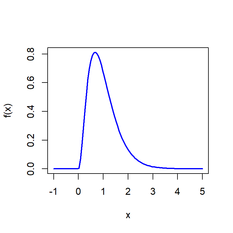
f =function(x){g(x)/val}curve(f(x), -1, 5, col ="blue", lwd =2)integrate(f, lower =0, upper =Inf)
1 with absolute error < 6.6e-06
Figure 4.13: The shape of the PDF \(f(x)\) which is obtained from the function \(g(x)\), after dividing by the constant \(M\), which is the area under the function \(g(x)\). Using the integrate() function, it is verified that \(f(x)\) is indeed a PDF.
Exercises - I
Check whether the following functions are PDF or not. - \(f(x) = \begin{cases} 0, ~~~~~~~~x<0 \\\frac{1}{(1+x)^2}, 0\le x<\infty\end{cases}\). -
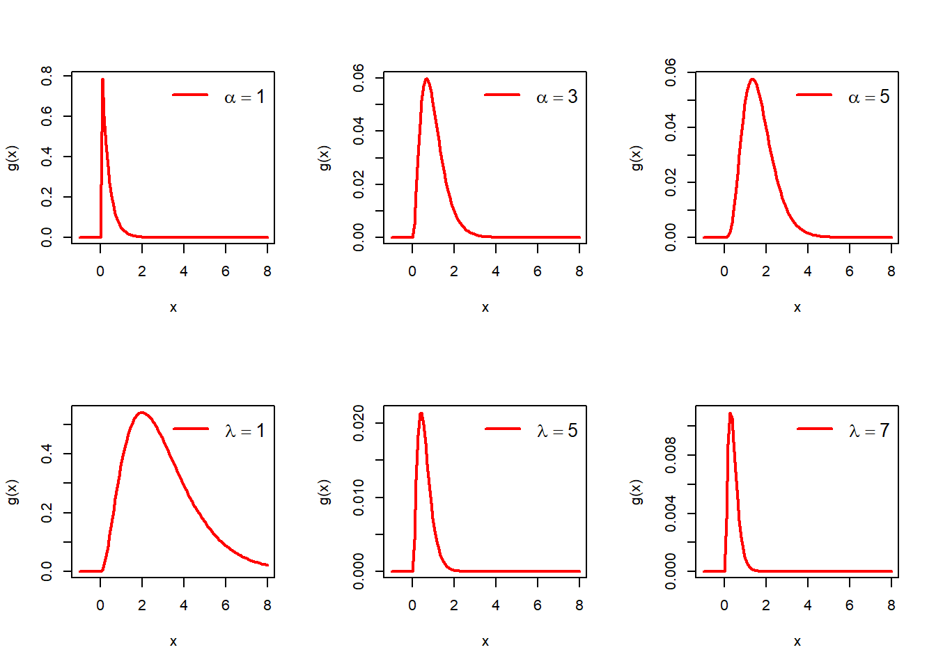
Let us expand the scope of this problem. Consider the following choice of \(g(x)\): \[g(x) = e^{-\lambda x} x^{\alpha - 1}, 0<x<\infty\] and zero otherwise.
alpha =3lambda =3M =gamma(alpha)/lambda^alphag =function(x){exp(-lambda*x)*x^(alpha -1)*(0<x)}f =function(x){ # define the PDFg(x)/M}par(mfrow =c(2,3))alpha_vals =c(1,3,5) # filling up first rowlambda =3for (alpha in alpha_vals) {curve(g(x), -1, 8, col ="red", lwd =2)legend("topright", legend =bquote(alpha == .(alpha)),bty ="n", cex =1.3, lwd =2, col ="red")}alpha =3lambda_vals =c(1,5,7)for (lambda in lambda_vals) {curve(g(x), -1, 8, col ="red", lwd =2)legend("topright", legend =bquote(lambda == .(lambda)),bty ="n", cex =1.3, lwd =2, col ="red")}
Figure 4.14: The shape of the fucntion \(g(x)\) for different choices of \(\alpha\) and \(\lambda\).
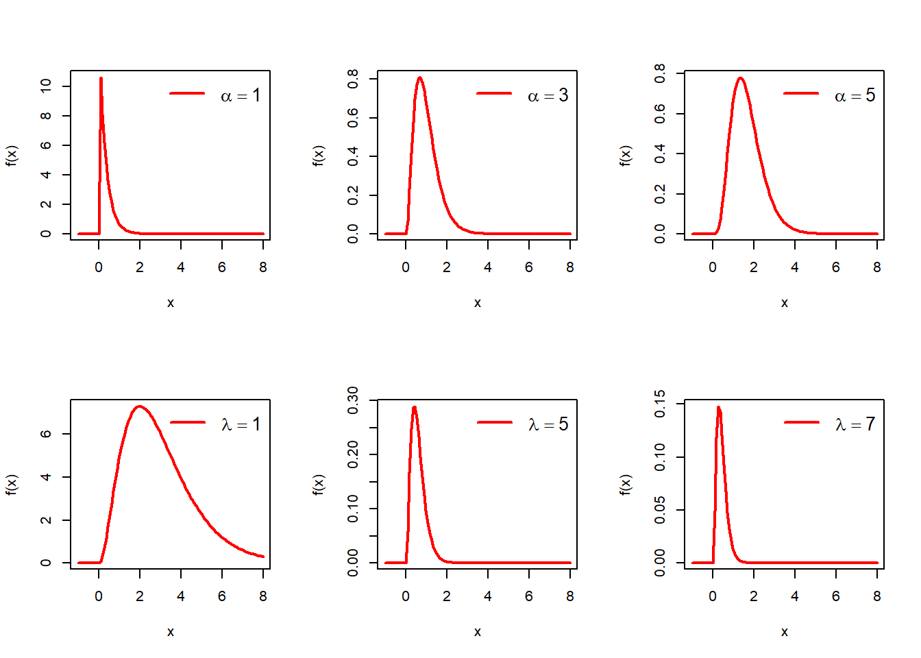
In the following, code, we convert the function \(g(x)\) to a PDF \(f(x)\). Students can identify that the integral can be converted to gamma integral and \[\int_0^{\infty} g(x)dx = \frac{\Gamma(\alpha)}{\lambda^{\alpha}}.\] Therefore, the PDF obtained from \(g(x)\) is given by \[f(x) = \begin{cases} \frac{e^{-\lambda x}x^{\alpha-1}\lambda^{\alpha}}{\Gamma(\alpha)}, 0<x<\infty, \\ 0, \mbox{otherwise}\end{cases}\]
par(mfrow =c(2,3))alpha_vals =c(1,3,5) # filling up first rowlambda =3for (alpha in alpha_vals) {curve(f(x), -1, 8, col ="red", lwd =2)legend("topright", legend =bquote(alpha == .(alpha)),bty ="n", cex =1.3, lwd =2, col ="red")}alpha =3lambda_vals =c(1,5,7)for (lambda in lambda_vals) {curve(f(x), -1, 8, col ="red", lwd =2)legend("topright", legend =bquote(lambda == .(lambda)),bty ="n", cex =1.3, lwd =2, col ="red")}
Figure 4.15: The shape of the probability density function \(f(x)\) which is also known as the gamma distribution with parameters \(\alpha\) and \(\lambda\).
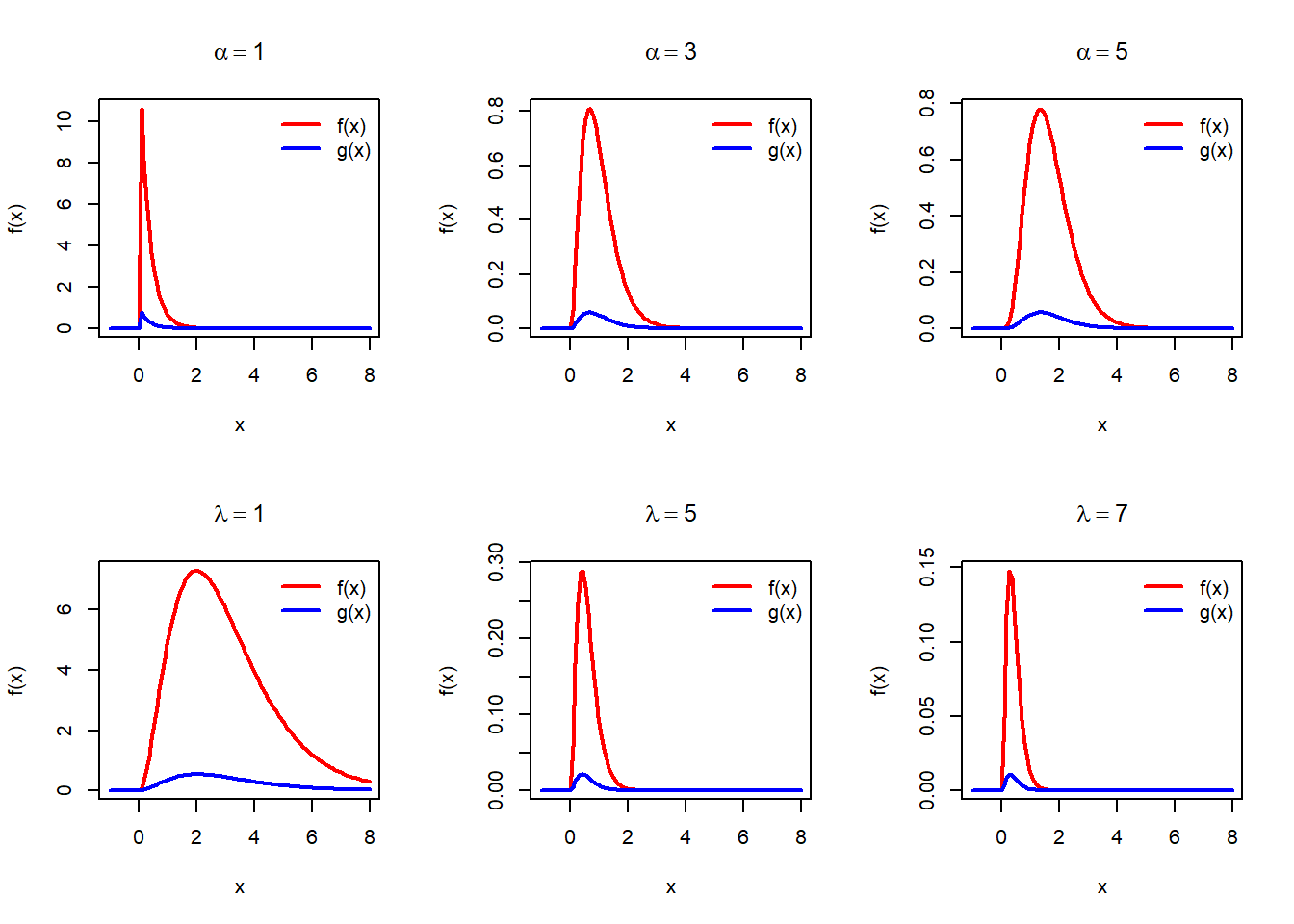
Let us plot \(f\) and \(g\) together
par(mfrow =c(2,3))alpha_vals =c(1,3,5) # filling up first rowlambda =3for (alpha in alpha_vals) {curve(f(x), -1, 8, col ="red", lwd =2, main =bquote(alpha == .(alpha)))curve(g(x), add =TRUE, col ="blue", lwd =2)legend("topright", legend =c("f(x)", "g(x)"), col =c("red", "blue"), lwd =c(2,2), bty ="n")}alpha =3lambda_vals =c(1,5,7)for (lambda in lambda_vals) {curve(f(x), -1, 8, col ="red", lwd =2, main =bquote(lambda == .(lambda)))curve(g(x), add =TRUE, col ="blue", lwd =2)legend("topright", legend =c("f(x)", "g(x)"), col =c("red", "blue"), lwd =c(2,2), bty ="n")}
mu =1sigma =1f =function(x){ (1/(sigma*sqrt(2*pi)))*exp(-(x-mu)^2/(2*sigma^2))}integrate(f, lower =-Inf, upper =+Inf)
1 with absolute error < 1.6e-05
f1 =function(x){ x*f(x)}integrate(f1, lower =-Inf, upper =+Inf)