7 Unbiased Estimation and Search for the Best Estimator
7.1 Search for the Best Unbiased Estimator
Till now we have learnt the following: We can compute the risk function of an estimator under different loss functions. If the computation is not possible to execute analytically, we know how to obtain the risk function by computer simulation. We have seen several examples, but we should keep in mind that always the simulation from the population distribution may not be an easy task. This idea will be explained later.
We can compute the maximum likelihood estimator of the parameters both analytically and numerically.
Still we are not in a position to decide whether we have obtained the best estimator which has the uniformly minimum risk against all estimators of the parameter. This is definitely a difficult task and we can not even imagine the universe of all possible estimators to get hold of one best estimator. In addition, even if we get hold of the best estimator, we are not really sure whether this is the unique one or not. Let us try to address these questions in this document.
7.2 Concentrating on Unbiased Estimators
To obtain the best estimator, we reduce our universe of all possible estimators to the set of all unbiased estimators. Suppose that we have a random sample of size \(n\) from the population PDF (PMF) \(f(x;\theta), \theta \in \Theta \subseteq \mathbb{R}\). An obvious consequence of having the class of unbiased estimators is that if \(\psi(X_1,\ldots,X_n)\) be an unbiased estimator of \(\theta\), then \(\mbox{E}_{\theta}\left(\psi\right)=\theta\) for all \(\theta\in \Theta\), which implies that under the squared error loss \[\mbox{E}_{\theta}\left(\psi_n-\theta\right)^2 = \mbox{E}_{\theta}\left(\psi-\mbox{E}_{\theta}\left(\psi_n\right)\right)^2 = Var_{\theta}(\psi_n).\] We keep the subscript \(n\) to emphasize the important role of sample size in studying the properties of the estimator. Therefore, for two unbiased estimators \(\psi_n'\) and \(\psi_n''\), \(\psi_n'\) will be a better estimator of \(\theta\) if \[Var_{\theta}(\psi_n')\le Var_{\theta}(\psi_n''), \mbox{ for all }\theta.\]
7.2.1 Uniformly Minimum Variance Unbiased Estimator
Let \(X_1,X_2,\ldots,X_n\) be a random sample of size \(n\) from the population PDF (PMF) \(f(x|\theta)\). Suppose we are interested in estimating \(g(\theta)\), a function of \(\theta\). An estimator \(\psi_n^*(X_1,\ldots,X_n)\) of \(g(\theta)\) is defined to be a uniformly minimum variance unbiased estimator of \(g(\theta)\) if \(\mbox{E}_{\theta}\left(\psi_n^*\right)=g(\theta)\) for all \(\theta \in \Theta\), that is, \(\psi_n^*\) is unbiased and \(Var_{\theta}\left(\psi_n^*\right)\le Var_{\theta}\left(\psi_n\right)\) for any other estimator \(\psi_n(X_1,\ldots,X_n)\) of \(g(\theta)\) which satisfies \(\mbox{E}_{\theta}\left(\psi_n\right)=g(\theta)\) for all \(\theta\in \Theta\).
7.3 Search for the minimum bound
In general we may not be always interested in estimating the parameter \(\theta\), rather we may be interested in estimating some function of the parameter \(g(\theta)\), say. For example, suppose a random sample of size \(n\) is available from the exponential distribution with rate parameter \(\lambda\) and we are interested in estimator \(\mbox{P}(X>1) = e^{-\lambda} = g(\lambda)\). The next discussion is generalized for estimating some function of the parameter \(g(\theta)\).
In search of the best estimator for \(g(\theta)\), some function of the parameter \(\theta\), we first try to find the least possible risk attained by any unbiased estimator of \(g(\theta)\) under squared error loss function. In other words, we want to compute a lower bound (sharp) for the variance of any unbiased estimator \(\psi\) of \(g(\theta)\).
7.3.1 Cramer-Rao Inequality
Suppose that \(X_1, X_2, \ldots,X_n\) be a random sample (not necessarily IID) of size \(n\) from the population PDF (PMF) \(f(x|\theta)\) and let \(\psi(\mathbf{X})\) be any estimator satisfying \[\frac{d}{d\theta}\mbox{E}_{\theta}(\psi(\mathbf{X}))=\int_{\chi} \frac{\partial}{\partial \theta}[\psi(\mathbf{X})f(\mathbf{x}|\theta)]d\mathbf{x}\] and \[Var_{\theta}\left(\psi(\mathbf{X})\right)<\infty,\] then \[Var_{\theta}\left(\psi_n(\mathbf{X})\right)\ge \frac{\left(\frac{d}{d\theta}\mbox{E}_{\theta}(\psi(\mathbf{X}))\right)^2}{\mbox{E}_{\theta}\left(\left(\frac{\partial}{\partial \theta}\log f(\mathbf{X}|\theta)\right)^2\right)}.\]
If the assumptions of the Cramer-Rao inequality are satisfied and, additionally, if \(X_1,X_2,\ldots,X_n\) are IID with PDF \(f(x|\theta)\), then \[Var_{\theta}\psi(\mathbf{X})\ge \frac{\left(\frac{d}{d\theta}\mbox{E}_{\theta}(\psi(\mathbf{X}))\right)^2}{n\mbox{E}_{\theta}\left(\left(\frac{\partial}{\partial \theta}\log f(X|\theta)\right)^2\right)}\]
Consider estimating the mean parameter \(\beta\) from the exponential PDF given by \(f(x) = \frac{1}{\beta}e^{-\frac{x}{\beta}}, 0<x<\infty\) and \(\beta\in(0,\infty)\). In this case \(g(\beta) = \beta\). Consider the MLE \(\overline{X_n}\) which is an unbiased estimator of \(\beta\) and \(Var_{\beta}\left(\overline{X_n}\right) = \frac{\beta^2}{n}\). Let us compute the CR bound for any unbiased estimator of \(\beta\). The denominator in the expression for C-R bound is computed below: \[\begin{eqnarray} n\mbox{E}_{\beta}\left(\left(\frac{\partial}{\partial \beta}\log f(X|\beta)\right)^2\right) &=& n\mbox{E}_{\beta}\left(\frac{\partial}{\partial \beta}\left(-\log \beta - \frac{X}{\beta}\right)\right)^2\\ &=& n\mbox{E}_{\beta}\left(-\frac{1}{\beta}+\frac{X}{\beta^2}\right)^2 = \frac{n}{\beta^4}\mbox{E}_{\beta}\left(X-\beta\right)^2 \\ &=& \frac{n \beta^2}{\beta^4} = \frac{n}{\beta^2}. \end{eqnarray}\] Therefore, the C-R bound is \(\frac{\beta^2}{n}\) and it is equal to \(Var_{\beta}\left(\overline{X_n}\right)\). Therefore, \(\overline{X_n}\) must be the UMVUE.
7.3.2 When C-R bound does not hold
Suppose that we have a random sample of size \(n\) from the following PDF \[f(x|\theta) = \begin{cases} \frac{2x}{\theta^2}, 0<x<\theta \\ 0,~~\mbox{otherwise}. \end{cases}\]
- Show that the MLE of \(\theta\) is \(Y_n = \max(X_1,\ldots,X_n)\).
- The MLE is not unbiased as \(\mbox{E}_{\theta}(Y_n) = \frac{2n\theta}{2n+1} \ne \theta\) for all \(\theta \in (0,\infty)\). However, \[\mbox{Bias}_{\theta}(Y_n) = \mbox{E}_{\theta}(Y_n)-\theta = -\frac{\theta}{2n+1}\to 0.\] as \(n\to \infty\). Therefore, MLE is asymptotically unbiased.
- However, we can obtain an unbiased estimator which is a function of \(Y_n\) as \(\psi_n = \frac{2n+1}{2n}Y_n\), then \[\mbox{E}_{\theta}\left(\psi_n\right) = \frac{2n+1}{2n}\times \frac{2n}{2n+1} \theta = \theta.\]
- The variance of \(\psi_n\) is obtained as follows:
- \(\mbox{E}_{\theta}\left(Y_n^2\right) = \frac{2n}{2n+2}\theta^2\).
- \(Var_{\theta}\left(Y_n\right) = \mbox{E}_{\theta}\left(Y_n^2\right) - \left(\mbox{E}_{\theta}(Y_n)\right)^2= \frac{n\theta^2}{(n+1)(2n+1)^2}\).
- \(Var_{\theta}\left(\psi_n\right) = \left(\frac{2n+1}{2n}\right)^2 Var_{\theta}\left(Y_n\right) = \frac{\theta^2}{4n(n+1)}\).
- Compute the C-R bound to verify that it is equal to \(\frac{\theta^2}{4n}\).
In the above problem, it is surprising to see that \[Var_{\theta}(\psi_n) = \frac{\theta^2}{4n(n+1)}<\frac{\theta^2}{4n} = \mbox{C-R bound}.\]
- Check that the required condition which allows the interchange of the derivative with respect to parameter \(\theta\) and the expectation does not satisfy for the given PDF.
- The result can be generalized further to observe that the support of the distribution depends on the unknown parameter \(\theta\), which is \((0,\theta)\). For such distributions, the criteria involving C-R lower bound can not be utilized to identify the best unbiased estimator. In fact, when the support depends on the parameter, C-R bound theorem does not work.
- Most of the book contains the \(\mbox{Uniform}(0,\theta)\) example to demonstrate the above exception, but, here we have a different example and you are encouraged to execute the above task. In line with this concept, one can actually test this using computer simulation as well. We can simulate the risk function of \(\psi_n^*\) using simulation and check that it completely lies below the C-R bound. One can use the probability integral transform to simulate from the given PDF.
par(mfrow = c(1,3))
theta_vals = c(2,4)
n = 100
for(theta in theta_vals){
  u = runif(n = n, min = 0, max = 1)
  x = theta*sqrt(u)
  hist(x, probability = TRUE, main = bquote(theta == .(theta)), ylim = c(0, 2/theta+0.1), cex.main = 1.3)
  curve(2*x/(theta^2)*(0<x)*(x<theta), add = TRUE,
        col = "red", lwd = 2)
}
# simulation of risk function for n = 4
n = 4
theta_vals = seq(1,4, by = 0.1)
risk_vals = numeric(length = length(theta_vals))
M = 1000             # number of replications
for(i in 1:length(theta_vals)){
  theta = theta_vals[i]
  psi_n = numeric(length = M)
  loss_vals = numeric(length = M)
  for(j in 1:M){
    u = runif(n = n, min = 0, max = 1)
    x = theta*sqrt(u)
    psi_n[j] = ((2*n+1)/(2*n))*max(x)
    loss_vals[j] = (psi_n[j] - theta)^2
  }
  risk_vals[i] = mean(loss_vals)
}
plot(theta_vals, risk_vals, col = "red", pch = 19,
     cex = 1.3, ylim = c(0, max(theta_vals)^2/(4*n)),
     xlab = expression(theta), ylab = expression(R(psi[n],theta)), main = paste("n = ", n))
curve(x^2/(4*n*(n+1)), col = "blue", lwd = 2, add = TRUE)
curve(x^2/(4*n), add = TRUE, col = "magenta",
      lwd = 2, lty = 2)
legend("topleft", legend = c("C-R bound"),
       lty = 2, col = "magenta", lwd = 2, bty = "n")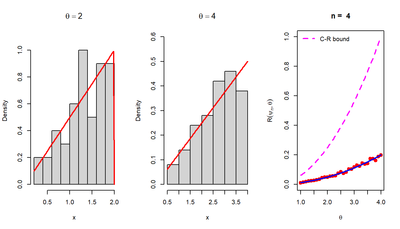
Therefore, we need to understand additional theories to characterize the UMVUE. We shall now introduce two important concepts, \(\texttt{Sufficient Statistics}\) and \(\texttt{Complete Statistics}\) which will help us address the gaps we encountered in characterizing the UMVUE.
7.3.3 Fisher Information Number
The following quantity which appears in the denominator of the lower bound for the variance of any unbiased estimator is known as the Fisher Information
\[\mbox{E}_{\theta}\left(\left(\frac{\partial}{\partial \theta}\log f(\mathbf{X}|\theta)\right)^2\right).\] This quantity tells us as the information number increases, we have more information about the parameter \(\theta\). An alternative computation for the Fisher Information can be eased by the following theorem.
If \(f(x|\theta)\) satisfies \[\frac{d}{d\theta}\mbox{E}_{\theta}\left(\frac{\partial}{\partial \theta} \log f\left(X|\theta\right)\right)= \int\frac{\partial}{\partial \theta}\left[\left(\frac{\partial}{\partial \theta}\log f(x|\theta)\right)f(x|\theta)\right]dx\], then \[\mbox{E}_{\theta}\left(\left(\frac{\partial}{\partial \theta}\log f(X|\theta)\right)^2\right) = -\mbox{E}_{\theta}\left(\frac{\partial^2}{\partial \theta^2}\log f\left(X|\theta\right)\right)\]
Let \(X_1,X_2,\ldots,X_n\) be independent and identically distributed random variables following \(f(x|\theta)\), and \(f(x|\theta)\) satisfies the conditions of the Cramer-Rao theorem. Let \(\mathcal{L}(\theta|\mathbf{x}) = \prod_{i=1}^nf(x_i|\theta)\) denote the likelihood function. If \(W(\mathbf{X}) = W(X_1,\ldots,X_n)\) be any unbiased estimator of \(g(\theta)\), then \(W(\mathbf{X})\) attains the Cramer-Rao Lower Bound if and only if \[a(\theta)[W(\mathbf{x})-g(\theta)]=\frac{\partial}{\partial \theta}\log \mathcal{L}(\theta|\mathbf{x}),\] for some function \(a(\theta)\).
7.4 Sufficient Statistics
Let \(X_1,X_2,\ldots,X_n\) be a random sample of size \(n\) from the PDF (PMF) \(f(x|\theta)\), where \(\theta\) may be a vector of parameters. A statistic \(T(X_1,\ldots,X_n)\) is said to be a sufficient statistic if the conditional distribution of \((X_1,\ldots,X_n)\) given \(T=t\) does not depend on \(\theta\) for any value \(t\) of \(T\).
If \(T(\mathbf{X})=T(X_1,\ldots,X_n)\) is a sufficient statistic for \(\theta\), then any inference about \(\theta\) should depend on the sample \(\mathbf{X}\) only through the value \(T(\mathbf{X})\). That is, if \(\mathbf{x}\) and \(\mathbf{y}\) are two sample points such that \(T(\mathbf{x})=T(\mathbf{y})\), then the inference about \(\theta\) should be the same whether \(\mathbf{X}=\mathbf{x}\) of \(\mathbf{Y} = \mathbf{y}\) is observed.
7.5 Exponential Family and minimal sufficient statistics
7.5.1 Exponential family of densities
A one-parameter family (the parameter \(\theta\in \Theta \subseteq \mathbb{R}\)) of PDF (PMF) \(f(x|\theta)\) that can be expressed as \[f(x|\theta) = a(\theta)b(x)e^{c(\theta)d(x)}\] for all \(x\in(-\infty,\infty)\) and for all \(\theta\in \Theta\), and for a suitable choice of functions \(a(\cdot)\), \(b(\cdot)\), \(c(\cdot)\) and \(d(\cdot)\) is defined to belong to the exponential family or exponential class.
If we have a random sample of size \(n\), from an exponential family, then the joint distribution of the data can be expressed as follow: \[\prod_{i=1}^nf(x_i|\theta)=(a(\theta))^n \left[\prod_{i=1}^nb(x_i)\right]\exp\left[c(\theta) \sum_{i=1}^nd(x_i)\right].\]
7.5.2 Worked examples
\(\mathcal{G}(\alpha,\beta)\) family: \[f(x|\alpha,\beta) = \frac{x^{\alpha-1}e^{-\frac{x}{\beta}}}{\Gamma(\alpha)\beta^{\alpha}}=a(\alpha,\beta)b(x)\exp\left[(\alpha-1) \log(x) + \left(-\frac{1}{\beta}\right)x\right],\] where \(a(\alpha,\beta) = \Gamma(\alpha)\beta^{\alpha}\), \(b(x)=1\), \(c_1(\alpha,\beta)=\alpha-1\), \(c_2(\alpha,\beta)-\frac{1}{\beta}\), \(d_1(x)=\log(x)\) and \(d_2(x) = x\). Therefore, \(\left(\sum_{i=1}^nX_i, \sum_{i=1}^n \log(X_i)\right)\) is jointly minimal sufficient for \((\alpha,\beta)\).
Show that the following PMFs belong to the exponential family and identify the corresponding minimal sufficient statistics
- \(\mbox{binomial}(n,\theta)\), \(n\) known.
- \(\mbox{Poisson}(\lambda)\)
- \(\mbox{Geometric}(p)\)
- \(\mbox{Discrete Uniform}\{1,2,\ldots,\theta\}\), \(\theta\in\{1,2,3,\ldots\}\).
Identify which of the following PDFs belong to the exponential family and identify the corresponding minimal sufficient statistics
- \(\mathcal{N}(\mu, \sigma^2)\)
- \(\mathcal{B}(a,b)\)
- \(\mathcal{G}(a,b)\)
- \(\mbox{Cauchy}(\mu,\sigma)\)
- \(\mbox{Uniform}(0,\theta)\)
According to the factorization criteria, \(\sum_{i=1}^nd\left(X_i\right)\) is a sufficient statistic for \(\theta\).
However, the above statement can be made much stronger in a sense that the above sufficient statistic \(\sum_{i=1}^n d(X_i)\) is in fact minimal sufficient.
7.5.3 \(k\)-parameter exponential family
A family of PDF (PMF) \(f(x|\theta_1,\ldots,\theta_k)\) that can be expressed as \[f\left(x|\theta_1,\ldots,\theta_k\right) = a(\theta_1,\ldots,\theta_k)b(x)\exp\left[\sum_{j=1}^nc_j(\theta_1,\ldots,\theta_k)d_j(x)\right]\] for suitable choice of functions \(a(\cdot,\ldots,\cdot)\), \(b(\cdot)\), \(c_j(\cdot,\ldots,\cdot)\) and \(d_j(\cdot)\), \(j=1,2,\ldots,k\) is defined to belong to the exponential family.
- The family of \(\mbox{Uniform(}0,\theta)\) does not belong to the exponential family.
- The statement cane is true in general. That is, any family of densities for which the range of the values were the density is non-negative depends of the parameter \(\theta\) does not belong the the exponential class.
7.5.4 Sufficiency and Unbiasedness
Let \(W\) be any unbiased estimator of \(g(\theta)\), and \(T\) be a sufficient statistic for \(\theta\). Define \(\phi(T) = \mbox{E}(W|T)\). Then,
- \(\mbox{E}_{\theta}\phi(T) = g(\theta)\).
- \(Var_{\theta}\phi(T) \le Var_{\theta} W\) for all \(\theta\). The above two conditions imply that \(\phi(T)\) is uniformly better unbiased estimator of \(g(\theta)\).
The Rao-Blackwell theorem states a very important fact that conditioning any unbiased estimator on a sufficient statistic will result in a uniform improvement, so we need to consider only statistics that are functions of a sufficient statistic in our search for the best estimators.
If \(W\) is a best unbiased estimator of \(g(\theta)\), then \(W\) is unique.
7.6 Complete Statistics
Let \(f(t|\theta)\) be a family of PDFs or PMFs for a statistic \(T(\mathbf{X})\). The family of probability distributions is called complete if \(\mbox{E}_{\theta}g(T)=0\) for all \(\theta\) implies \(\mbox{P}(g(X)=0) = 1\) for all \(\theta\). Equivalently, \(T(\mathbf{X})\) is a complete statistic.
7.6.1 Examples of Complete family
- Let \((X_1,X_2,\ldots,X_n)\) be iid \(\mbox{Uniform}(0,\theta)\) observations, \(0<\theta<\infty\). Then \(T(\mathbf{X}) = \max(X_1,\ldots,X_n)= X_{(n)}\) is a complete statistic.
- Let \(X_1,\ldots,X_n\) be a random sample from a population with PDF \[f(x|\theta)=\theta x^{\theta-1}, 0<x<1, 0<\theta<\infty.\] Find a complete sufficient statistics for \(\theta\).
- Let \(X_1,X_2,\ldots,X_n\) be IID with geometric distribution \[\mbox{P}_{\theta}(X=x)=\theta (1-\theta)^{x-1}. x=1,2,\ldots,~0<\theta<1.\] Show that \(\sum_{i=1}^nX_i\) is sufficient for \(\theta\), and find the family of distributions of \(\sum X_i\). Check whether the family is complete.
7.6.2 Complete statistics in the exponential family
Let \(X_1,X_2,\ldots,X_n\) be iid observations from an exponential family with PDF or PMF of the form \[f(x|\boldsymbol{\theta})=a(\boldsymbol{\theta})b(x)\exp\left(\sum_{j=1}^k c_j(\boldsymbol{\theta})d_j(x)\right),\] where \(\boldsymbol{\theta} = (\theta_1,\ldots,\theta_k)\). Then the statistic \[T(\mathbf{X})=\left(\sum_{i=1}^n d_1(X_i),\sum_{i=1}^n d_2(X_i),\ldots,\sum_{i=1}^n d_k(X_i)\right)\] is complete if \(\{(c_1(\boldsymbol{\theta}),c_2(\boldsymbol{\theta}),\ldots, c_k(\boldsymbol{\theta}))\colon \boldsymbol{\theta}\in \Theta\}\) contains an open set in \(\mathbb{R}^k\).
- If \(X_1,\ldots,X_n \sim \mathcal{N}\left(\theta,\theta^2\right)\). Here the parameter space \((\theta,\theta^2)\) does not contain a two-dimensional open set, as it consists of only the points on the parabola.
The following theorem delineates the connection between complete sufficiency of an unbiased estimator with the best unbiased estimator.
7.7 Best unbiased estimator
Let \(T\) be a complete sufficient statistic for the parameter \(\theta\), and let \(\phi(T)\) be any estimator based only on \(T\). Then \(\phi(T)\) is the unique best unbiased estimator of its expected value.
Let us see an illustrative example. Suppose \(X_1,X_2,\ldots,X_n\) be IID \(f(x|\theta)\), where \[f(x|\theta) = \theta x^{\theta-1}I_{(0,1)}(x), 0<\theta<\infty.\]
- First we observe that this PDF belongs to the exponential family as \[f(x|\theta) = \theta \times 1 \times \exp\left[(\theta -1)\log x\right] = a(\theta)b(x)\exp[c(\theta)d(x)]\]
- Therefore, \(\sum_{i=1}^n \log X_i\) is complete sufficient (in fact minimal) statistic for \(\theta\).
- Compute the MLE of \(\theta\): the likelihood function \(\mathcal{L}(\theta) = \theta^n \left(\prod_{i=1}^n x_i^{\theta-1}\right)\) and \[l(\theta) = \log \mathcal{L}(\theta) = n \log \theta + (\theta - 1)\sum_{i=1}^n\log X_i.\] Solving \(l'(\theta)=0\), we obtain the MLE of \(\theta\) as \[\widehat{\theta_n} =T_n= -\frac{n}{\sum_{i=1}^n\log X_i}.\]
- First let us check whether \(\widehat{\theta_n}\) is unbiased. We must note that the MLE is in fact a function \(T_n\), which is a complete sufficient statistic \(\sum_{i=1}^n\log X_i\). We obtain the sampling distribution of \(\widehat{\theta_n}\).
- (Step - I) Show that \(Y_i = -\log X_i \sim \mbox{Exponential}(\mbox{rate} = \theta)\).
- (Step - II) Show that \(Y = \sum_{i=1}^n Y_i= -\sum_{i=1}^n\log X_i \sim \mathcal{G}\left(\alpha = n, \beta = \frac{1}{\theta}\right)\).
- (Step - IV) Show that the PDF of \(\widehat{\theta_n}\) is given by \(f_{T_n}(z) = \frac{(n\theta)^ne^{-\frac{n\theta}{z}}}{\Gamma(n)z^{n+1}}, 0<z<\infty\).
- (Step - V) Show that \(\mbox{E}_{\theta}\left(T_n\right) = \frac{n\theta}{n-1}, n>1\). Therefore, \(T_n\) is not an unbiased estimator of \(\theta\).
- (Step - VI) We can get an unbiased estimator which is a function of \(T_n\), which is a function of a complete sufficient statistic as \(T_n^* = \frac{n-1}{n}T_n = -\frac{n-1}{\sum_{i=1}^n\log X_i}\). Therefore, \(T_n^*\) is the best unbiased estimator.
- (Step - VII) Compute the variance of \(T_n^*\)
- (Step - VIII) Compute the C-R bound for any unbiased estimator of \(\theta\) and check whether \(Var_{\theta}\left(T_n^*\right) = I_n(\theta)^{-1}\) for all \(\theta\in(0,\infty)\).